A proposed framework for assessing risk from less-than-lifetime exposures to carcinogens

Abstract

Quantitative methods for estimation of cancer risk have been developed for daily, lifetime human exposures. There are a variety of studies or methodologies available to address less-than-lifetime exposures. However, a common framework for evaluating risk from less-than-lifetime exposures (including short-term and/or intermittent exposures) does not exist, which could result in inconsistencies in risk assessment practice. To address this risk assessment need, a committee of the International Life Sciences Institute (ILSI) Health and Environmental Sciences Institute conducted a multisector workshop in late 2009 to discuss available literature, different methodologies, and a proposed framework. The proposed framework provides a decision tree and guidance for cancer risk assessments for less-than-lifetime exposures based on current knowledge of mode of action and dose-response. Available data from rodent studies and epidemiological studies involving less-than-lifetime exposures are considered, in addition to statistical approaches described in the literature for evaluating the impact of changing the dose rate and exposure duration for exposure to carcinogens. The decision tree also provides for scenarios in which an assumption of potential carcinogenicity is appropriate (e.g., based on structural alerts or genotoxicity data), but bioassay or other data are lacking from which a chemical-specific cancer potency can be determined. This paper presents an overview of the rationale for the workshop, reviews historical background, describes the proposed framework for assessing less-than-lifetime exposures to potential human carcinogens, and suggests next steps.

Keywords::

• Cancer risk assessment
• dose-rate correction factors (DRCFs)
• Haber’s Rule
• intermittent exposure
• less-than-lifetime exposure (LTL)
• short-term exposure
• threshold of toxicological concern (TTC)

Acknowledgments

The authors express their appreciation to the staff of Cantox Health Sciences International for preparing some of the analyses of the animal studies relating to time of exposure and cancer incidence with chemicals (see Appendix E).

Declaration of interest

The employment affiliations of the authors are shown on the first page. Six of the authors are employed by the following companies: Eli Lilly and Company, ExxonMobil Biomedical Sciences, Inc., Johnson and Johnson Pharmaceuticals, Kraft Foods, The Proctor & Gamble Company, and Unilever. These companies develop, manufacture, and market products, some of which are regulated by government agencies that may, in the future, consider the use of the proposed framework for assessing risk from less-than-lifetime exposures to carcinogens as described in this paper. Seven of the authors are employed by government agencies that may use the proposed framework in discharging their legal and scientific responsibilities. Four of the authors are employed by academic institutions. One of the authors is an independent consultant (Kirkland Consulting) whose company provides scientific advice to public and private organizations. One of the authors is an employee of the ILSI Health and Environmental Sciences Institute (HESI). The mission of HESI, a nonprofit organization, is to stimulate and support scientific research and educational programs that contribute to the identification and resolution of health and environmental issues of concern to the public, scientific community, government agencies, and industry (www.hesiglobal.org). HESI provides a unique, objective forum for in-depth dialogue among scientists from around the world affiliated with academia, industry, and public sector research and regulatory organizations (both governmental and nongovernmental). Industry members provide primary financial support for HESI programs, but HESI also receives financial and in-kind support from a variety of US and international government agencies and other scientific organizations.

The authors had sole responsibility for the writing and content of the paper. The views and opinions expressed in the paper are those of the authors, and do not necessarily reflect the views of the authors’ employers; the opinions or policies of the US EPA, the US FDA, WHO, or RIVM (National Institute for Public Health and the Environment, The Netherlands); or the participants in the December 1–3, 2009, workshop (Figure 2). Mention of trade names does not constitute endorsement. None of the authors has recently or is currently involved as an expert witness in litigation or formal government rule-making on the subject of this paper. None of the authors received financial support or an honorarium in the preparation of this paper.

The authors gratefully acknowledge the in-kind support provided by the following sponsors of the December 1–3, 2009, workshop:

• US EPA National Center for Computational Toxicology

• US EPA National Health and Environmental Effects Research Laboratory

The authors gratefully acknowledge the financial support provided by the following sponsors of the December 1–3, 2009, workshop:

• Eli Lilly and Company

• ExxonMobil Biomedical Sciences, Inc.

• Georgia Pacific LLC

• ILSI Europe

• ILSI North America Task Force on Food and Chemical Safety

• Johnson & Johnson Pharmaceuticals

• NIH National Institute of Environmental Health Sciences

• The Procter & Gamble Company

• Society of Toxicology Food Safety Specialty Section

• Society of Toxicology Regulatory and Safety Evaluation Specialty Section

• Society of Toxicology Risk Assessment Specialty Section

• Unilever

• US FDA Center for Food Safety and Applied Nutrition

Appendix A. Cancer biology

The development of neoplasms in both experimental animals and humans is a complex, multistep process, involving a series of genetic and epigenetic alterations. The process consists of two distinct sequences: initiation (or neoplastic transformation), followed by promotion (or neoplastic development).

The sequence of initiation involves conversion of a normal cell to an initiated or transformed neoplastic cell. This process is almost certainly the consequence of abnormalities in gene function, which can be inherited, spontaneous, or induced by carcinogens. Such changes in gene function can result from mutation or permanent epigenetic changes. These typically, but not necessarily, require DNA replication and hence the critical target cells for carcinogens are principally the renewing stem cells in tissues. However, in light of the ability of adult cells to reprogram into induced pluripotent cells, it is certainly possible, if not likely, that adult, differentiated cells also can serve as progenitors for cancer cells.

Spontaneous mutations can arise from DNA hydrolysis, errors in DNA synthesis, or errors of repair processes acting on endogenously modified DNA. Induced mutations result from chemical modification of DNA, which is not corrected by DNA damage repair systems and, consequently, during DNA replication, gives rise to structural alterations in DNA. Epigenetic changes in DNA expression can be produced by several alterations, including modification of the pattern of DNA methylation.

In the evolution of a neoplastic cell, focal preneoplastic populations usually precede the appearance of neoplasms and are considered to be the progenitors of the neoplastic cells that constitute tumors. Those preneoplastic cells that are not necessarily committed to progress to neoplasms presumably lack all the requisite genetic changes that characterize neoplastic cells. In contrast, fully transformed cells are neoplastic and will form neoplasms under permissive conditions. Preneoplastic lesions in both rodents and humans often express the same phenotypic abnormalities found in neoplastic cells, which are a consequence of alterations in gene function. Thus, preneoplastic lesions have been demonstrated to carry gene mutations found in the tumors that develop in association with the precursor lesions. The development of preneoplastic lesions can be enhanced by agents referred to as tumor promoters. Also, increased cell proliferation and impaired DNA repair capability may be involved in rendering preneoplastic cells more susceptible to transformation with continued carcinogen exposure.

The mutations, as well as epigenetic changes, that underlie transformation are primarily those in growth control genes, the proto-oncogenes and tumor suppressor genes, or genes that regulate expression of these genes. Over 100 oncogenes and 30 tumor suppressor genes have been identified. Proto-oncogenes function as positive regulators of cell proliferation, which are converted to activated oncogenes by a variety of types of genetic alteration. Tumor suppressor genes are negative regulators of proliferation and are inactivated by several types of genetic alteration. Epigenetic mechanisms of gene silencing include under- or overmethylation of DNA and alterations in histone acetylation. Some of these genetic changes may occur in the genesis of the neoplastic cell, whereas others emerge during further neoplastic development. At least four to seven critical alterations in function of growth control genes are implicated in the development of human cancer cells, whereas fewer appear sufficient in rodent cells. In fully neoplastic cells, very large numbers of alterations in methylation and mutations accumulate, likely due to defects in fidelity of DNA replication.

In the second sequence of oncogenesis, tumor promotion involves facilitation of the growth of both preneoplastic cells and neoplastic cells through a variety of mechanisms, mainly epigenetic. Promoters include both endogenous chemicals, such as hormones, and exogenous chemicals, all of which show specificity in the species and organs affected. Their main action in the sequence of transformation is to facilitate clonal expansion of responsive preneoplastic cells. Eventually, the preneoplastic cells with the requisite genetic alterations for selective growth emerge as populations in which transformation to neoplastic cells has occurred.

In neoplastic development, the neoplastic cell or population generated during initiation proliferates disproportionately to the surrounding tissue, thereby achieving clonal expansion to eventually form a neoplasm. Progressive growth can result from either enhanced capacity for proliferation or reduced programmed cell death, referred to as apoptosis.

Neoplasms may be well differentiated, i.e., they express morphological and functional features of the cells of their tissue of origin, and are benign in their biologic behavior. Qualitative changes in the biologic behavior of a neoplasm toward malignancy are known as progression and are likely due to accumulation of changes in gene function. Progression may be the consequence of a mutator phenotype, which introduces mutations in replicating neoplastic cells, or a methylator phenotype, which introduces epigenetic alterations, adding to those occurring spontaneously or induced by carcinogen exposure. The basis for the mutator phenotype can involve reduced fidelity of DNA replication and diminished DNA repair processes. Progression leads to the development of malignant neoplasms with the ability to invade and metastasize. Ultimately, most, if not all, neoplasms develop structural or numerical chromosomal alterations.

The essential alteration in neoplastic cells is dysregulation of growth control. This stems either from the activity of the gene products of oncogenes, which regulate cell survival and proliferation, or from functional loss of the gene products of tumor suppressor genes, which inhibit cell proliferation. Thus, the progressive growth of neoplasms is due to an imbalance of a higher percentage of dysregulated neoplastic cells traversing the cell cycle (i.e., a high growth fraction) exceeding the percentage leaving the cell cycle to the resting state (G₀), differentiation, or apoptosis.

The MOA of carcinogens in the two sequences of neoplasia is reflected in their dose-response characteristics and determines their potential to produce human effects.

A number of review articles on cancer biology exist. These include Berenblum (1974), Croce (2008), Esteller (2007), Goodman and Watson (2002), Kamendulis and Klaunig (2008), Lopez et al. (2009), and Vogelstein and Kinzler (2004).

Appendix B. Cancer risk assessment: History and further developments

B.1. International approaches to cancer risk assessment

The Joint Food and Agriculture Organization/World Health Organization (FAO/WHO) Expert Committee on Food Additives (JECFA), first formed in 1956 to evaluate the safety of food additives, has considered unavoidable food contaminants since 1972. With respect to carcinogenic contaminants, addressed since 1984 when considering low-level migration from food packaging material, the Committee did not consider it appropriate to establish tolerable intake levels (i.e., reference doses, tolerable daily intake [TDI]). In such cases the Committee did not perform a formal risk assessment, but after consideration of the hazard profile of the compound as well as estimated human exposure, recommended that human exposure should be reduced to the lowest level technologically achievable. This is often referred to as the ALARA principle—to reduce exposure to “as low as reasonably achievable,” which is the recommendation given for risk management actions. Subsequently a differentiation has been made between contaminants that act through a mode of action for which there is assumed to be a threshold and for which a tolerable intake level can be established, and those where a threshold of action cannot be assumed, mainly genotoxic carcinogens.

The International Programme on Chemical Safety (IPCS) has also developed a systematic framework to evaluate the cancer mode of action in rodents and assess the human relevance of such tumors. The framework for the animal cancer mode of action was published in 2001 and expanded to human relevance assessment in 2006 (see below for further details). This framework is applied in the practical risk assessment work of international expert bodies such as JECFA and the Joint FAO/WHO Meeting on Pesticide Residues (JMPR).

The WHO program to establish guidelines for drinking water quality assesses the risk of chemical contaminants. For compounds considered to be genotoxic, guidelines are generally derived using the linearized multistage model. In such cases the guideline values represent the concentration in drinking water associated with an estimated upper bound excess life-time cancer risk of 10⁻⁵ (assuming a lifetime of 70 years and a daily consumption of 1.5 L).

B.1.1. JECFA and EFSA: MOE approach

At its 64th meeting (WHO, 2006), JECFA gave further consideration to the assessment of contaminants in food with genotoxic and carcinogenic properties. The ALARA approach, described above, provides no insights into the actual, or even relative, potency of the compound, nor does it take any account of estimated human exposure, and therefore does not allow risk managers to prioritize actions. JECFA considered several options and decided to use the margin of exposure (MOE) approach. The MOE comprises two components: (1) the benchmark dose at the lower confidence limit (BMDL), and (2) estimated intake of the contaminant. The BMDL is obtained using a curve-fitting approach that extrapolates a 10% response from toxicology data and an upper or lower bound at the 95% confidence interval (Crump, 1984b). It is often used in risk assessment as the point of departure for threshold-based assessments (using uncertainty factors) or nonthreshold assessments (using linear extrapolation). In the case of the MOE, one simply takes the ratio of the BMDL over exposure intake, enabling the provision of (semi)quantitative advice to risk managers on such contaminants. There is less of a concern for situations where there are high ratios, whereas situations where the ratios are lower may require risk management action, including recalls of food products. Subsequently, the European Food Safety Authority (EFSA) published a scientific opinion on the application of the MOE approach (EFSA, 2005), proposing a similar approach to that of JECFA. The MOE takes into account the potency of the carcinogen through dose-response modeling and the derivation of the BMDL, as well as estimated human exposure. It provides a relative indication of the level of human health concern but not an estimation of the actual cancer risk. Recently, ILSI Europe, in collaboration with WHO and EFSA, reached a very similar conclusion on the utility of the MOE approach for food-borne genotoxic carcinogens (Benford et al., 2010). This assessment included a number of case studies that explored the strengths and weaknesses of using such an approach.

B.2. National approaches

B.2.1. Cancer risk assessment at the US Environmental Protection Agency (US EPA)

Albert (1994) provided an informative review of cancer risk assessment as it developed during the 1970s and 1980s at the then nascent US EPA. Albert describes how President Nixon declared the “war on cancer” in 1970 and how, at that time, epidemiological evidence suggested that 60–90% of cancers were caused by environmental factors. Thus, in the early years of US EPA, there was much enthusiasm for the idea that a better understanding of cancer risk and regulation based on this understanding could potentially relieve much of society’s cancer burden.

Albert noted that it was appropriate for a Federal agency to adopt a conservative, risk-averse policy in the absence of a fuller understanding of carcinogenic mechanisms. The need for a clear distinction between hazard identification and quantitative risk assessment was recognized early on, as was the challenge of extrapolation from doses used in rodent bioassays to the much lower levels of exposure typically encountered by people. The US EPA published draft guidelines for cancer risk assessment in 1976: “Interim Procedures and Guidelines for Health Risk and Economic Impact Assessments of Suspected Carcinogens” (US EPA, 1976). The assumption that carcinogen dose-response curves were low-dose linear was a key element of these guidelines. This assumption was thought to be consistent with the concept that mutations cause cancer, and a single molecule could conceivably cause DNA damage leading to mutation, a theory that originated in the field of radiation risk assessment (Appendix J). The guidelines also accepted the use of carcinogenicity data from bioassays of laboratory animals and the use of maximum tolerated doses for practical reasons, i.e., because human epidemiological data were usually insufficient and because studies with adequate statistical power to detect very low response rates, such as 1 in 10⁶, are not feasible. Commitment to quantitative risk assessment required use of a model to formalize the low-dose extrapolation. This was another key feature of the draft guidelines, providing the capability of predicting dose associated with any particular risk level, even for risks far below those seen experimentally. Although many possible models were considered, in the end, the precedent established by the US Atomic Energy Commission for use of the linear-no-threshold model to assess risk in radiation carcinogenesis was used to justify the same approach for chemical carcinogenesis.

The draft guidelines were finalized in 1986 (US EPA, 1986), with the main assumptions regarding quantitative risk assessment, low-dose linearity, use of data from laboratory animals, and use of high doses unchanged, though the finalized guidelines were also influenced by the “Red Book” on risk assessment published by the National Academies of Sciences (NAS) in 1983 (NRC, 1983).

Beginning in the late 1970s, and then increasingly throughout the 1980s and onwards, research on toxicological mechanisms started to identify nonlinear and, in some cases, threshold dose-response behaviors that were not consistent with the linearity assumptions of the 1986 Guidelines. For example, physiologically based pharmacokinetic (PBPK) modeling was used to show that the low-dose cancer risk of methylene chloride (MC) was considerably lower than indicated by linear extrapolation from the tumor data due to dose-dependent nonlinearities in MC bioactivation (Andersen et al., 1987). Detailed studies of the biotransformation and toxicity of chloroform provided compelling evidence that the rodent tumors caused by this compound were secondary to chronic cytolethality and regenerative cellular proliferation, whereas related studies showed a lack of direct interaction with DNA (Butterworth and Bogdanffy, 1999). The weight of the evidence thus suggests a threshold in the dose-response for chloroform carcinogenicity, as the key precursor event, cytolethality, is a threshold phenomenon. These and many other studies motivated revision of the 1986 Guidelines, a process that began in the early 1990s, progressed through several drafts, and was finalized in 2005 (US EPA, 2005a).

The 2005 Guidelines formally acknowledged that the shapes of carcinogen dose-response curves are determined by pharmacokinetic and pharmacodynamic (PK/PD) mechanisms. Thus, models containing appropriate descriptions of these mechanisms would provide predictions of risk at relevant levels of exposure with arguably less uncertainty than statistical models. The new Guidelines introduced the concepts of MOA and key event, which define realistic requirements for data generation in support of the dose-response modeling, and a “mode of action framework,” which provides specific guidance for evaluation of the data in support of the hypothesized MOA. An option for linear extrapolation is retained for instances wherein the data support an MOA consistent with low-dose linearity (for example, a mutagenic MOA). Low-dose linearity is also the EPA default approach used when no MOA can be determined.

Although the 2005 Guidelines are current as of the preparation of this paper, some recent developments indicate significant sentiment for use of low-dose linear extrapolation, even if the MOA is arguably highly nonlinear or even thresholded (NRC, 2009). The crux of the argument is that population heterogeneity will tend to linearize any dose-response curve, because individuals will vary in the dose at which nonlinearities or thresholds occur (NRC, 2009). Others have expressed skepticism that data-driven dose-response modeling can ever be refined to the point of actually being less uncertain than statistically based extrapolation (Crump et al., 2010). Thus, although the 2005 Guidelines specifically encouraged mechanistic research and associated computational modeling in support of dose-response assessment, it is not at this time clear if this will in fact be the approach preferred by regulatory risk assessors in the future.

B.2.2. Health Canada—T₀₅

Health Canada approaches cancer risk assessment by calculating a TD₀₅/TC₀₅ (i.e., the dose or concentration associated with a 5% increase in tumor incidence above background). For mutagenic carcinogens, it is assumed that there is some probability of harm to human health at any level of exposure (i.e., there is no threshold). However, Health Canada does not generally advocate low-dose linear extrapolation as a risk assessment method to calculate a negligible risk level. Rather, the TD₀₅/TC₀₅ is then compared with exposure levels. If the ratio between exposure and the TD₀₅/TC₀₅ is less than 2 × 10⁻⁶, there is little need for further action. If the ratio is 2 × 10⁻⁴ or greater, there is a high priority for further action. Values in between are of moderate priority. The methods of Health Canada are described further in the Agency’s document “Health-Based Tolerable Daily Intakes/Concentrations and Tumorigenic Doses/Concentrations for Priority Substances” (Health Canada, 1996).

B.3. The Cancer Potency Database (CPDB)—TD₅₀

The Cancer Potency Database (CPDB) (available online: http://potency.berkeley.edu/) was established in the 1980s, and includes data from the largest number of rodent bioassays of any other web site (Gold et al., 1984, 1991, 1992, 1999, 2005). The measure of carcinogenic potency used is the TD₅₀, or the dose resulting in a 50% tumor increase over background (Peto et al., 1984; Sawyer et al., 1984). The CPDB has been used in a wide variety of applications, mainly because of its large size, including 1547 chemicals (as of April 30, 2010). For each chemical, a TD₅₀ value for each species was developed, which was the most potent value from all organ sites considered statistically significant. If there was more than one value for the same organ site, the harmonic mean TD₅₀ was reported. Most notable from its applications, TD₅₀ values were used to derive the TTC for potential carcinogens (Appendix C) (Kroes et al., 2004; Rulis, 1986). Risk assessment using the TD₅₀ has included two approaches: (1) straight linear extrapolation from a 50% response, or (2) 0.87/TD₅₀ = q1 × (cancer potency slope curve), cancer potency estimate used by the US EPA (Gaylor and Gold, 1995).

B.4. Advances in cancer risk assessment: incorporating mode of action and other data into the risk assessment process

The testing of chemicals for carcinogenicity has been markedly influenced by the National Cancer Institute (NCI) and the National Toxicology Program (NTP) of the US, established in the 1960s. Following the establishment of NTP, much development work was based on the premise that carcinogens were, in general, DNA reactive (Weisburger, 1983) and as a consequence, much effort was spent in developing short-term tests of genotoxicity—specifically, of mutagenicity. A major outcome was the Salmonella bacterial mutation assay of Ames (1973). A large majority of chemicals (>90%) proved to be DNA reactive and mutagenic in the Ames test and led to the view summed up in the title of the seminal paper by Ames (1973): “Carcinogens are mutagens: a simple test system combining liver homogenates for activation and bacteria for detection.”

However, as chemicals with greater structural diversity were tested in the NTP program, it became apparent that a number of substances, with no structural or experimental evidence for DNA reactivity or genotoxicity, were capable of inducing a carcinogenic response. Indeed, the proportion of these substances that were carcinogenic was similar to that of DNA-reactive substances, but the profile of tumors produced was not the same (Fung et al., 1995). In the ensuing years, it has become abundantly apparent that chemicals can cause cancer by a variety of mechanisms, in addition to genotoxicity. A further important finding was that as a consequence of the specific physiological or biochemical processes involved, some of these mechanisms (modes of action) are not relevant to humans, due to fundamental species differences in these processes, e.g., the presence of alpha-2μ-globulin uniquely in the male rat, so that the renal carcinogenicity of certain compounds dependent on interaction with this protein is not relevant to humans (MacDonald and Scribner, 1999).

In general, such nongenotoxic carcinogens act by inducing sustained proliferation, either directly through a trophic stimulus or indirectly by inducing a proliferative response as a consequence of cell death (see Meek et al., 2003; Boobis et al., 2006; WHO, 2007). As discussed above, this will favor the selection of cells that either have been, or become, initiated due to spontaneous replication errors or induced damage, e.g., by reactive oxygen species (Ames and Gold, 1997; Nordstrand et al., 2007).

There is experimental and mechanistic evidence that such nongenotoxic carcinogens exhibit a threshold in their dose-response curves below which adaptive and repair processes operate to prevent irreversible effects (see Boobis et al., 2009), and that exposure must be sustained because of both reversibility and the low chance of spontaneous or induced initiation of a cell. This is true both when the underlying process is spontaneous misreplication and through DNA damage induced via secondary mediators (Chan et al., 2009). In the latter situation, a threshold concentration of the carcinogen will be necessary to induce mediator release, e.g., through inflammation (Butterworth and Bogdanffy, 1999). Although there is, at least theoretically, potential for a single molecule of a DNA-reactive compound to induce mutation on a single exposure, and hence to initiate carcinogenicity (US EPA, 2005a), this is being increasingly questioned (e.g., Williams et al., 2004). For example, it takes no account of the requirement of promotion and other post-initiation events, and there is now good evidence that processes such as DNA repair are very efficient, with considerable redundancy in the pathways (Larsen et al., 2007; Hsieh and Yamane, 2008; Yonekura et al., 2009).

Many cancer risk assessment guidelines now take into account these developments in the understanding of chemical carcinogenesis. For example, the current US EPA guidelines for cancer risk assessment (US EPA, 2005a) state quite clearly that “[t]he use of mode of action in the assessment of potential carcinogens is a main focus of these cancer guidelines.” Where sufficient data are available to determine the mode of action and to conclude that it is not linear at low doses, nonlinear extrapolation can be used. In effect, this is analogous to the use of safety or uncertainty factors, with a customary default of 100 applied to the point of departure, e.g., no observed adverse effect level (NOAEL) or BMDL₁₀. A similar approach is taken by many other authorities and risk assessment groups, such as the UK Committee on Carcinogenicity (2004), the joint WHO/JMPR expert groups (JMPR and JECFA) and by EFSA. For example, the EFSA Scientific Panel on Plant Health, Plant Protection Products and their Residues (EFSA, 2003) concluded that although it was not possible to establish unequivocally the mode of action for liver tumors by mepanipyrin, there was sufficient information to conclude that the dose-response exhibited a threshold and recommended that risk assessment should proceed accordingly.

A mode of action comprises a series of key events, i.e., observable and quantifiable effects that are necessary, though individually probably not sufficient, to cause cancer. An example of a key event would be the metabolic activation of chloroform to phosgene. Although this is a necessary event in the hepatocarcinogenesis of chloroform, on its own it is not sufficient. Tumor induction by chloroform requires subsequent sustained cytotoxicity and regenerative hyperplasia—also key events (Boobis et al., 2009). A key event may be either kinetic or dynamic. It has been recognized, either explicitly or implicitly, in many cancer guidelines, that characterization of the dose- and time-response relationships for key events can inform interspecies extrapolation of cancer risk. This may be qualitative, so that species differences are so great that risk to humans is considered negligible (Meek et al., 2003) or it may be quantitative, e.g., permitting the use of chemical-specific adjustment factors, rather than defaults (Meek et al., 2002; WHO, 2005). An example of such a framework is provided in Figure 4 (adapted from Boobis et al., 2006).

Figure 4.  Example of a framework for the assessment of the human relevance of a cancer mode of action identified in experimental animals (see Boobis et al., 2006).

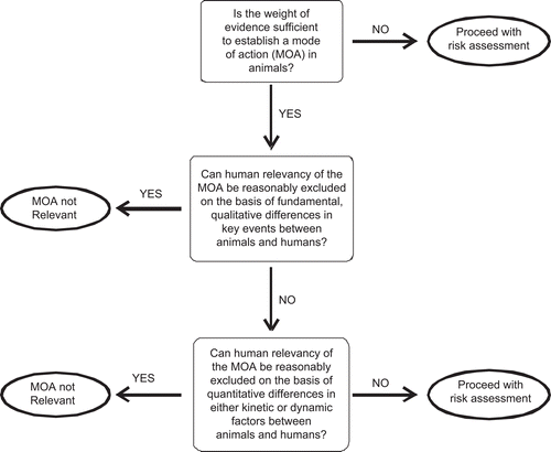
A mode of action is an operational description, in terms of key events, of the kinetic and dynamic processes that underlie the carcinogenic response under a defined set of circumstances, e.g., route of administration, cell type, sex, strain, and species (Boobis et al., 2006; WHO, 2007). Although it is likely that the same mode of action will apply to a range of circumstances, suitable evidence for this would need to be provided. A common situation where a mixed mode of action is proposed is where there is evidence of both genotoxicity and cytotoxicity, e.g., with formaldehyde (McGregor et al., 2006). However, application of the mode of action framework may enable a conclusion to be reached as to the importance of these processes, e.g., by detailed analysis of dose- and time-responses of the key events. It could also be that it is not possible to determine beyond reasonable doubt as to whether one or both processes is involved. However, as indicated above, the analysis may provide sufficient information to enable a conclusion to be reached about the nature of the dose-response curve and/or quantitative interspecies differences.

Mixed modes of action are sometimes proposed when in reality the mode of action changes with dose, i.e., there is a dose transition (Slikker et al., 2004a). As indicated above, it is important to consider the extent to which the circumstances of a study are generalizable, with dose as with other aspects of study design. In applying the mode of action framework, a key consideration is dose-response concordance of key events, both between each other and with the carcinogenic effect. This should reveal any inconsistency with dose. If such inconsistency is identified, it might be necessary to undertake mode of action analysis for different dose ranges, over which there is a carcinogenic response.

Appendix C. Other methods for estimating cancer risk when chemical-specific data are limited

As the number of chemicals requiring risk assessments along with the pressure to limit animal testing continues to increase, many assessments will have limited or no carcinogenicity data. Given this reality, methodologies are becoming available that provide practical tools when data are not available but exposure is low, including (1) extrapolation from an in vivo mutagenicity study; (2) utilization of data derived from subchronic repeat-dose toxicity studies and dividing by a defined safety margin; (3) QSAR and read-across (SAR) approaches; and (4) the threshold of toxicological concern (TTC).

1. Short-term in vitro mutagenicity assays, such as the Ames assay, are typically used to predict cancer hazard, but have not been a basis for successful quantitative risk estimation (Travis et al., 1990). For a group of 34 diverse carcinogens, Sanner and Dybing (2005) found a linear correlation between the lowest effective dose (LED) in an in vivo genotoxic test and with the cancer T₂₅ (the chronic daily dose which corresponds to 25% of the animals developing tumors above background at a specific tissue site). There was a good correlation between the LED and T₂₅, with a correlation coefficient (r²) of.7. The median of the ratio LED/T₂₅ was found to be 1.05 and it was also found that the ratio fell in the range 0.21 to 9.2 for 90% of the substances studied. Based on these results, the authors suggested that LED for in vivo mutation assays could be used as a basis for regulation of mutagens in cases where the substance has not been studied in long-term carcinogenicity studies. However, this method has not yet been employed by regulatory agencies.

2. Data from short-term studies provide the advantage of quicker results with fewer animals. The maximum tolerated dose (MTD) method is used in the design of dose-selection for carcinogenicity studies, where a correlation can be made between the MTD and carcinogenic potency. Gaylor and Gold (1995) showed that dividing the MTD derived from a 90-day study by a factor of 740,000 could provide an estimate of a virtually safe dose (VSD), or the chronic dose resulting in a 1 in 1 million excess cancer risk. They found that for 96% of the NCI/NTP carcinogens, the calculated VSD was within a factor of 10 of this ratio. Similarly, a simple estimate of an LED-10 can be calculated from an MTD (available, or estimated from a subchronic study) as: LED-10 = MTD/7 (Gaylor and Gold, 1998). The LED-10 is defined as the dose resulting in a 10% increase in tumors at the lower 95th percent confidence interval; the acceptable dose can then be linearly extrapolated from the LED-10.

3. (Q)SAR and “in silico” technologies have been used successfully in prediction of hazards based on chemical structure but are also being used for risk assessment (Benfenati et al., 2009). In general, QSAR models have provided good results for class-specific predictions (Benigni et al., 2009). Reasonable success was obtained using a Classification and Regression Tree (CART) QSAR model to predict a TD₅₀—an estimate of cancer potency or the dose that would result in a 50% probability of developing cancer over background (Venkatapathy et al., 2009). There has been a recent effort to apply in silico tools to predict carcinogenic potency based on structure to be used for assessment of risk for genotoxic impurities in pharmaceuticals (Bercu et al., 2010). This approach combined a classification method to define “potent” and “not-potent” compounds with a quantitative assessment of cancer potency for the “not-potent” compounds. The results were conservative, with a high sensitivity (86–88%) and lower specificity (36–85%) for classifications of consensus models in rats and mice. Further, a majority (86–88%) of quantitative predictions were ≤ a 5× ratio of predicted TD₅₀s/actual TD₅₀s (test set), indicating that it was rare to underpredict carcinogenic potency beyond normal variability of a cancer bioassay (10×) (Gaylor et al., 1993; Gaylor and Gold, 1995). “Read across” SAR techniques use structural analogs from well-studied compounds to provide risk estimation when data is limited for the chemical in question (Wu et al., 2010). Research in (Q)SAR for cancer risk assessment continues to improve and as such may be more useful for decision making.

4. The TTC has been used as a practical default when no toxicity information is known for a compound. In the Delaney Clause (1958) for the Amendment to the Food, Drugs, and Cosmetic Act (1938), it was initially stipulated that no food or color additive could be approved if found to cause cancer in man or animals. The concept of a TTC was established by the Food and Drug Administration (FDA)/Center for Food Safety and Applied Nutrition (CFSAN) in 1995 (US FDA, 1995) as the threshold of regulation for food packaging leachables. The threshold of regulation was considered an exposure of “de minimis” carcinogenic risk. This was based on an assessment of 343 carcinogens from a carcinogenic potency database (CPDB) and was derived from the probability distribution of carcinogenic potencies of those compounds (Rulis, 1986). Subsequent analyses of an expanded database of more than 700 carcinogens further confirmed the threshold (Kroes et al., 2004; Fiori and Meyerhoff, 2002). An exposure of 1.5 µg/day was established as the threshold of regulation (21 CFR 170.39—Threshold of regulation for substances used in food-contact articles), such that a compound with unknown toxicity would be of de minimis risk for potential carcinogenicity.

The TTC was expanded to provide a noncarcinogenic risk assessment for compounds where data are limited. A database of compounds with noncarcinogenic effects was developed and linked to an SAR (Cramer) classification scheme (Cramer et al., 1978; Kroes et al., 2004; Munro et al., 1996). No observed effect levels (NOELs) were identified for these compounds. The lower 5th percentile chronic NOEL from a distribution of available toxicology studies for each class of compounds was selected, and a 100-fold safety factor was applied to this value. If a subchronic NOEL was identified, then a 300-fold safety factor was applied. Thresholds were developed for three structural categories: Class 1—1800 µg/day (“Substances of simple chemical structure and efficient modes of metabolism that would suggest a low order of oral toxicity”); Class 2—540 µg/day (“Substances that are in a structural class in which there is less knowledge of the metabolism, pharmacology and toxicology, but for which there is no clear indication of toxicity”); and Class 3—90 µg/day (“Substances of a chemical structure that permit no strong initial presumption of safety, or that may even suggest significant toxicity”) (Munro et al., 1996). This classification scheme is applied within a decision tree approach by the Joint FAO/WHO Expert Committee on Food Additives (JECFA) to evaluate the safety of food flavoring substances (Munro et al., 1999). Software (e.g., Toxtree) has been developed to facilitate the Cramer structural classification of compounds (Patlewicz et al., 2008). Although these thresholds are suitable for noncarcinogens, a more conservative estimate is often times applied for compounds with carcinogenic potential.

The TTC value developed using carcinogenicity data assumed two factors: (1) the probability that a compound is carcinogenic; and (2) the accepted excess cancer risk (Munro et al., 1999). The first assumption depends on how much data are available for a compound. For example, it is assumed that there is about a 5–10% chance that a random compound would result in a carcinogenic response (Fung et al., 1995). The probability increases if the compound is positive for genotoxicity, depending on the assay(s) used (Barlow et al., 2001). The second assumption of acceptable cancer excess cancer risk can vary from organization to organization depending on risk management practices. Typically, the accepted excess cancer risk for a carcinogen ranges from 10⁻⁵ to 10⁻⁶ for substances when the general population may be exposed to low levels (Kroes et al., 2004; Müller et al., 2006).

Kroes et al. (2004) extended the TTC concept for compounds with a structural alert for genotoxicity. Compounds from the CPDB were linearly extrapolated to negligible risk values from their corresponding TD₅₀s. From this analysis, it was concluded that exposure to 0.15 µg/day was associated with a high probability of not exceeding a 1 in 1 million excess cancer risk. Others have adopted 1.5 µg/day as the acceptable TTC for genotoxic compounds; this dose represents a 1 in 100,000 excess cancer risk (Müller et al., 2006). The CPDB was further analyzed based on structural class and certain structures were labeled as the cohorts of concern (COC) (e.g., aflatoxins, N-nitrosos, azoxys) (Kroes et al., 2004). These compounds are of higher carcinogenic potency; thus, the TTC was not a low enough dose to maintain a negligible excess cancer risk. However, it should be noted that the TTC conservatively assumes that a genotoxic compound will likely result in a carcinogenic response, and that there is no threshold for effect. Further it assumes that the genotoxic (or potentially genotoxic) compound is of higher carcinogenic potency than nongenotoxic compounds (Parodi et al., 1991; Cheeseman et al., 1999).

Special care must be used when applying the TTC. First, careful consideration must be made to determine if the compound of interest would be contained within the chemical space of the 700 compounds in the database used to establish the TTC. Because the TTC was developed for oral exposures, other considerations must be made when applying this approach to other routes of exposure (Kroes et al., 2007). Both carcinogenic and noncarcinogenic endpoints should be considered for a compound when applying the TTC, which may require different thresholds. Haber’s Rule (e.g., linearly redistributing lifetime exposure during short durations) has been applied to the TTC, with a description of its use for regulatory guidances in Appendix G.

Appendix D. Haber’s Rule (background and references to applications in cancer risk assessment)

Haber’s Rule states that the incidence and/or severity of an adverse effect is a function of the total exposure to a potentially toxic chemical, i.e., C × T = k. Haber based this rule on his acute inhalation toxicity studies on the lethality time-concentration relationship of some gases used as weapons in World War I (Haber, 1924). He observed that the product of exposure concentration and time resulted in a constant lethal response. The basic concept is nowadays extended to other routes of exposure and to longer time intervals (Gaylor, 2000; Miller et al., 2000). Haber’s Rule is also a basic concept in cancer risk assessment for genotoxic carcinogens in which the carcinogenic potential of a chemical is assumed to be related to the cumulative dose. The applicability of Haber’s Rule herein is considered justified by the basic philosophy that the carcinogenic process is a stochastic event. Thus, the probability of a tumor is considered to be proportional to the total number of molecules at the target site and thus proportional to the total or cumulative dose.

Although Haber’s Rule has been applied in a variety of situations, there were still many situations that appeared not to comply with Haber’s Rule. Rozman and Doull (2000a, 2000b) extended the concept of time in the process of toxicity. They assumed that Haber’s Rule under isodosic or isotemporal conditions represents a fundamental law of toxicology and, thus, that there should be no exceptions to it. Apparent deviations could then be understood or explained (and should be studied) by understanding the half-lives for kinetics and dynamics (Rozman and Doull, 2001).

Rozman and Doull (2000a) reasoned that although dose is a “pure variable,” the component of “time” in the process of toxicity is a complex phenomenon comprised of different aspects, each with its own time scales. They distinguished three independent time scales: the frequency of exposure, the kinetic time scale, and the dynamic time scale. The kinetic time scale is an intrinsic property of the organism, whereas the dynamic time scale is considered to be an intrinsic property of the compound. The third time scale, frequency of exposure, is independent of the two other time scales. In continuous exposure, the kinetic and the dynamic time scales are forced to become synchronized, thereby diminishing the number of time scales to be dealt with to one. This synchronization will also occur when the frequency of exposure becomes so high that it becomes indistinguishable from continuous exposure. For compounds with either very short dynamic or kinetic half-lives, such a synchronization will be achieved by continuous exposure only.

All three determinants have their own time course, which is the result of supply and removal. The time course of a compound in the body (kinetic time scale) is determined by the ratio between the absorption rate and the elimination rate, with the latter considered to be the rate-determining or rate-limiting phase. By analogy, the dynamic phase is considered to be a function of injury and recovery rate, with the latter considered to be rate-determining (or rate-limiting) (Rozman and Doull, 2000a). The kinetic half-life will dominate the overall process of toxicity if it is longer than the dynamic half-life. In case of a compound with a slow recovery (i.e., the effect recovery half-life is longer than the kinetic half-life), the dynamic half-life will dominate the dynamics of an effect. They proposed a decision tree-type analysis to identify the critical steps in the toxicity of chemicals, i.e., to identify the most critical time scale. They illustrated this concept with a few cases in a subsequent paper (Rozman and Doull, 2001).

Miller et al. (2000) acknowledged the complexity of time as a contributor to toxicity and recognized that the above-mentioned three time scales are fundamental aspects in understanding the process of toxicity. However, they contended that Haber’s Rule is merely a special member of a family of power functions described by C^α × T^β = k₁ (viz. when α = β = 1) and that using this general power law will be more effective to study the relative contributions of the different time scales and dose, and will provide a better insight than the concept as discussed by Rozman and Doull. The general power law can be rewritten as Cⁿ × T = k₂ (with n = α/β), which is used within several frameworks in emergency response planning (e.g., US EPA Acute Exposure Guideline Level [AEGL] program) and for land use planning purposes for the prediction of health effects following (single) acute exposures. However, this concept has predominantly been studied in acute respiratory exposure situations within a limited time frame and with mortality as the endpoint. Although within the AEGL program, lifetime carcinogenic risks for respiratory exposures are extrapolated to exposure durations of less than 24 hours (always with a default n = 1 independent of the n derived or estimated for mortality), it still needs to be further investigated whether the general power law also holds true for extrapolations of lifetime exposures to shorter time intervals for genotoxic carcinogens. Druckrey (1967) studied the carcinogenicity of a large number of nitrosamines and concluded that the latency to cancer could best be described by C × Tⁿ = k with n > 1.

The importance of the above considerations for risk assessment of LTL exposures to carcinogens is evident but they are difficult to address and to incorporate into a generally applicable scheme for this purpose. The concept presented by Rozman and Doull, including their decision tree-type analysis, might provide a valuable scheme along which the evaluation of a carcinogenic risk for shorter than lifetime exposures might proceed. However, it requires a detailed insight into the mode of action that will often be absent. For instance, it is important to know whether the parent compound itself or a metabolite is responsible for the carcinogenic response. Within the concept of Rozman and Doull, metabolism of the parent compound will belong to the kinetic elimination phase if the parent compound is carcinogenic, but to the kinetic supply phase if the metabolite is responsible for the tumor induction.

The importance of this issue is connected to the recovery rate of effects, which in turn depends on the rate-limiting processes in dynamics and kinetics. When there is no recovery at all, it is only the accumulated dose that will count (Haber’s Rule). However, as the kinetic and dynamic half-lives become shorter and shorter, the frequency of the external exposure will become more and more important. Furthermore, the kinetic and dynamic supply and elimination phases may be very different in short-term exposure to high doses as compared to lifetime exposure to low doses.

A further issue that is not accounted for by Haber’s Rule, but that should be considered, is the age at time of exposure. A specific dose might appear to be more potent at a relatively susceptible age than at other ages. For instance, analyses of female atomic bomb survivors showed that females with exposure age under 20 had higher relative risk of breast cancer than females exposed at higher age (Land et al., 2003), which may also be the case in exposure to chemical carcinogens (see Appendix J). In the process of risk assessment, this aspect should be covered by application of a DRCF, but it is mentioned here because it should be considered when studying data for the applicability of Haber’s Rule.

In addition, it should be realized that a lifetime human risk estimate is often based on the total carcinogenic response at the end of a 2-year animal experiment. However, in the present context, in order to address or derive some relationship between dose and time, the actual time-to-tumor would be a more appropriate parameter to consider. If, for instance, in an animal experiment a tumor becomes manifest after 18 months, the cumulative dose causing tumor formation should be calculated from this 18-month exposure period. Inclusion into the LCD of the dose administered after the tumor becomes manifest will then lead to an underestimation of the carcinogenic potency of a chemical.

At present, the best way forward appears to be a pragmatic approach, because the available kinetic and dynamic data will often be too limited to adequately address the issues raised above. If appropriate data are available these can be evaluated case by case and used to deviate from the default approach.

The default basis for carcinogenic risk assessment for less-than-lifetime exposure is a lifetime risk estimate such as a “virtually safe dose” (VSD) that is associated with a defined risk (e.g., 1 in 10⁶). This lifetime risk estimate is derived through linear extrapolation from an animal experiment or human epidemiological data. By default, linear extrapolation means that the exponent α in the general power function C^α × T^β = k is set equal to 1. Because time is a constant (lifetime animal to lifetime human) when extrapolating an observed tumor incidence in a 2-year animal experiment to a human VSD, the exponent β in the general power law could in theory deviate from 1. However, the basic philosophy of the carcinogenic process being a stochastic event means that the total dose is expressed as C × T = k, with both α and β equal to 1. Thus the VSD is usually derived using Haber’s Rule. Therefore, for reasons of consistency, it appears most appropriate to similarly apply Haber’s Rule when extrapolating the VSD to a shorter, uninterrupted period of exposure.

Appendix E. Data to consider in developing methods for assessing less-than-lifetime cancer risk

E.1. Introduction

A series of less-than-lifetime, compared to lifetime, studies with chemicals has been conducted by the National Toxicology Program (NTP) in the US. These NTP “stop-exposure” studies follow the same general protocol as the standard 2-year bioassay, but the animals are exposed for a more limited time, followed by an exposure-free period for the remainder of the 2-year study so that the animals are the same age when they are sacrificed. The doses were varied so as to either have equal or nonequal doses over the total lifetime of the animals. A limited analysis of the empirical data from the NTP rodent bioassay “stop-exposure” studies was conducted by Halmes et al. (2000). This analysis showed that, indeed, the chemical potency could be increased or decreased by condensing the dose into a short exposure period, but most changes were within a factor of 2-fold.

E.2. Stop-exposure studies of carcinogens carried out by the NTP

Test agents were chosen on the basis of human exposure, level of production, and chemical structure. These studies primarily assessed carcinogenesis in rats or mice, following chemical exposure for approximately 2 years; however, several reports included a stop-exposure phase in which some animals were exposed to the chemical for a shorter period, followed by an exposure-free period for the remainder of the 2-year study. Within each study, animals with the same level of exposure from all groups were sacrificed at the same age and assessed for tumor incidence.

E.3. Studies using equal daily doses

In studies with six chemicals, equal daily doses in the stop-exposure and chronic exposure groups were employed, resulting in a higher overall exposure in the chronic exposure group. The relationship between duration of exposure and tumor incidences varied depending on the chemical and the tumor type. All six of the compounds tested positive for genetic toxicity. The results of these studies are summarized in Table 1 and are described below.

Table 1.  Comparison of stop-exposure versus continuous exposure studies in animals: Equal daily doses.

Based on the assumption that the relationship between length of exposure and tumor incidence is linear, the expected percent tumor incidence in the stop-exposure groups was calculated as follows:

The effects on tumor incidence for short-term compared to continuous exposure for the NTP studies on chemicals are summarized in Table 1.

In addition to the studies conducted by the NTP, Kari et al. (1993) reported tumor incidences in mice exposed to 2000 ppm methylene chloride for durations ranging from 26 to 104 weeks. To examine the influence of age of exposure on the induction tumors, mice in the stop-exposure groups were exposed to methylene chloride either early or late in life. In mice treated for 26 or 52 weeks early in life, the observed incidences of lung and liver tumors were higher than expected based on the incidences reported in chronically exposed animals. Similar observed and expected values were found in mice exposed for 78 weeks. In contrast, lower-than-expected lung and liver tumor incidences were reported in mice exposed to methylene chloride later in life for 26, 52, or 78 weeks, with the exception of liver tumors in mice exposed for 26 weeks. These results support the idea that the life stage in which exposure occurs may influence the relationship between duration of exposure and tumor response.

Similarly, Drew et al. (1983) evaluated the relationship between age and exposure duration for cancer induction by vinyl chloride in rats, mice, and hamsters. In all three species, exposures were most effective in the induction of tumors when started early in life. Rats with early initial exposure had an increased incidence of hemangiosarcomas, hepatocellular carcinomas, and mammary gland carcinomas, whereas rats held for 12 months prior to exposure did not have an increase in any of these tumors. Similar results were seen for hamsters and mice (with the first 6 months of dosing being most critical in mice).

Littlefield et al. (1979) conducted a study commonly referred to as the “megamouse study” exposing Balb/c female mice to 2-acetylaminofluorene (2-AAF) to study the dose-response to liver and bladder tumors over a period of up to 33 months, with continuous treatment periods of 9, 12, 15, and 24 months. A comparison of the expected compared to the observed lifetime tumor incidences in the bladder and the liver showed that the shorter-term exposures to 2-AAF produced a less than expected incidence of bladder neoplasms at the only dose producing a dose-related tumor response (150 ppm), whereas the liver tumor incidence was increased at all doses where there was a response, with an inverse trend for tumor increase, with time of exposure. This lifetime adjusted inverse tumor incidence increase, related to time of exposure was equally apparent at the lowest exposure level (60 ppm) as at the highest (150 ppm). The steps critical to the development of liver tumors were considered to be sufficiently established by 9 months of continuous exposure, and that no further exposure was required. In fact, further exposure reduced the lifetime adjusted incidence of tumors, presumably by increasing apoptosis or by direct toxicity to transformed cells. It is therefore possible to have a lifetime adjusted increased incidence of one type of tumor (liver) related to less-than-lifetime exposure and a decreased lifetime adjusted incidence of another tumor (bladder) in the same study with the same carcinogen. All of the dose-related effects of lifetime adjustment of the tumor incidence in this study were within a 2-fold difference of the 2-year continuous exposure incidence (Littlefield et al., 1979).

E.4. Studies using unequal daily doses

Several stop-exposure studies did not include equal daily doses when comparing effects of stop-exposure to chronic exposure. Instead, they utilized larger daily doses in the stop-exposure groups, often resulting in a time-averaged daily dose equivalent to the daily exposure in the continuous exposure groups. Thus, the total amount of the carcinogenic agent received by the animal over its life span was equal in both groups. 2,2-Bis(bromomethyl)-1,3-propanediol, furan, methyleugenol and o-nitroanisole tested positive for genotoxicity, whereas weakly positive results for chromosomal aberrations and sister chromatid exchanges were reported for pentachlorophenol. Results of these studies are shown in Table 2, and are described below.

Table 2.  Stop-exposure versus continuous exposure studies in animals: Equivalent/similar time-averaged doses.

The time-averaged dose is calculated as follows:

The results of these comparisons are shown in Table 2 and have been reviewed in detail by Halmes et al. (2000). Generally the treatment of animals in the short-term increased the incidence of tumors found at the end of the study period compared to the animals continuously exposed.

E.5. Examination of total dose and time of exposure using diethylnitrosamine

Druckrey et al. (1963) conducted a study to investigate the carcinogenic potential of diethylnitrosamine (DENA) in rats. Constant doses of DENA (0.075, 0.15, 0.3, 0.6, 1.2, 2.4, 4.8, 9.6, and 14.2 mg/kg body weight/day) were administered in drinking water to BD II rats over their lifetimes. The total dose required to induce carcinomas in 50% of animals (D₅₀) declined with decreased daily dose and increased induction time. Specifically, the D₅₀ was 64 mg/kg in rats treated with 0.075 mg/kg DENA per day for 840 days, and was 965 mg/kg in rats treated with 14.2 mg/kg per day for 68 days. Therefore, exposure to low doses over an extended period of time is more potent than high-dose exposure for a shorter duration.

The significance of the relationship between exposure duration and dose administered in determining risk was summarised by Druckrey (1967) as:

where d is the daily dose, t is the length of time in days required for the induction of cancer in 50% of treated animals, and n is the tangent of the angle of increase in a plot on a double log system of the daily dose with the average induction time in 50% of the animals. In the case of DENA, n = 2.3, indicating that carcinogenic activity increases by more than the square of the induction time. In other carcinogens studied by Druckrey, the value of the exponent n is predominantly between 2 and 4, and always greater than 1. Because time has an exponent in the equation, it appears to drive the carcinogenic response more than the daily dose. Therefore, short-term exposures are less potent than long-term exposures, assuming the same cumulative lifetime dose.

E.6. Summary of less-than-lifetime animal exposure studies

The available stop-exposure studies demonstrate that for some test agents, short-term exposures are no more potent in causing tumor formation than lifetime exposures, but for other carcinogens, short-term exposure may be associated with an increase in cancer risk relative to chronic exposure. Statistical methods were used to evaluate the degree to which adjusted stop-exposures led to calculated unit risks that were higher or lower than those calculated from studies involving chronic exposure. However, in a number of studies, the daily dose administered to the animals was much greater in the stop-exposure groups. Increases in daily exposure may influence the mode of action for tumor induction, influencing cellular responses to the chemical agent, including metabolism of the agent, detoxification mechanisms, DNA repair activity and the initiation of programmed cell death in response to high levels of DNA damage, as well as increasing the rate of cell proliferation in some organs due to cytotoxicity (liver and kidney in particularly).

In some of the stop-exposure groups, the duration of treatment was up to 78 weeks, which is 75% of a 2-year lifetime. Assuming a lifetime of 70 years in humans, this corresponds to 52.5 years of exposure. Even the shortest exposure period in the stop-exposure studies (13 weeks) does not reflect short-term exposure in humans, as it corresponds to a human exposure time of 8–9 years. Therefore, the observed increase in potency of some stop-exposure treatments may not be predictive of human short-term exposure. Essentially, the animal data from the stop-exposure studies is equivocal with respect to support of the hypothesis that linear extrapolation of chronic risk to calculated risk for short-term exposures represents a conservative approach. Even if these examples were to reflect a real human high-dose exposure situation, the deviation from linear extrapolation was never found to be more than 8-fold in terms of observed short-term tumor incidence compared to the expected incidence of tumors from the lifetime exposure data. It is noted that this is within the range of variability that has been estimated for the rodent bioassay (Gaylor et al., 1993). For the stop and continuous exposure studies reviewed by Halmes (Halmes et al., 2000), the situation was different. For most of the genotoxic carcinogens that they reviewed, the difference in potency was within 1 order of magnitude; however, the two exceptions were three cancer endpoints in the animal studies with 2,2-bis(bromomethyl)-1,3-propanediol, which were up to 50-fold different, and one cancer endpoint for 1,3-butadiene, where there was a 100-fold difference in potency.

E.7. Single-dose exposure to carcinogens

The conclusions from the analysis of the single exposure carcinogen database (Calabrese and Blain, 1999), using approximately 800 chemicals and including around 5500 studies, were that a single exposure to a chemical could be sufficient to cause cancer over a lifetime, and that the hazard correlated with exposures to chemical carcinogens where the exposure was for an effective lifetime. The dose of a chemical administered was fractionated over a lifetime, and the tumor response was compared to the response, after only a single dose. Eight chemicals gave a lower tumor incidence after a single dose than after dose fractionation, whereas five gave a higher incidence and another nine chemicals produced similar results. There was no apparent relationship to the class of chemical, its structure, or the known genotoxicity across this spectrum of results.

E.8. Further evaluation of the single-dose carcinogen database

The potency of genotoxic carcinogens has been compared after single or short-term doses to further the suggestion that the Calabrese database could be informative about risk assessment for carcinogens (Calabrese and Blain, 1999).

Using this database a pilot study was prepared for the UK Committee on Carcinogenicity (2005) by the UK Department of Health Toxicology Unit (available at http://www.iacoc.org.uk/papers/documents/cc0619.pdf). This analysis derived T₂₅ values for 5 genotoxic carcinogens, i.e., dibenz(a,h)anthracene, N-nitrosodiethylamine, N-nitrosodimethylamine, methylnitrosourea, and benzo(a)pyrene, and compared the single dose potency to the carcinogenic potency from the chronic bioassay data.

The limitations of this approach were that most of the chronic values were obtained from oral dosing studies, whereas a range of routes had been used for the single dose exposures. There was no apparent correlation in the ranking of calculated acute T₂₅ values and chronic T₂₅ values for the five chemicals for which acute T₂₅ values could be calculated (Table 3).

Table 3.  Comparative data of the calculated chronic T₂₅ values with the calculated acute T₂₅ values.

The T₂₅ value normally relates to long-term exposure, which could include additional effects related to chronic cytotoxicity and repeated DNA repair, which contribute to the carcinogenic risk. Lifetime tumor incidence depends on the accumulation of risk and there is not necessarily going to be a correlation between the risk from acute exposure and that from chronic exposure due to the additional, sometimes thresholded factors contributing to the development of cancer.

E.9. Case studies comparing single and continuous exposures to carcinogens

Hehir et al. (1981) investigated the effects of a single exposure to vinyl chloride on carcinogenesis in the mouse lung. ICR mice were exposed for 1 hour to 50–50,000 ppm vinyl chloride by inhalation. The incidence of pulmonary adenomas at 8 and 18 months following exposure of mice to 500, 5000, or 50,000 ppm vinyl chloride increased compared to control mice, and some of the adenomas progressed to carcinomas (Table 4).

Table 4.  Histological examination of mice following a single exposure to vinyl chloride (Hehir et al., 1981).

The single exposure study with ICR mice was considered negative at 50 and 500 ppm-h, borderline at 5000 ppm-h, but did produce neoplastic lesions in the lung at 50,000 ppm-h. In multiple-exposure studies with vinyl chloride, A/J mice exposed to multiple doses of 50 ppm for 100 days 1 h/day or 500 ppm for 10 days 1 h/day for a total cumulative dose of vinyl chloride of 5000 ppm-h show a significant increased tumor incidence, but only at the higher dose level (Hehir et al., 1981).

The multiple exposure experiment at 50 and 500 ppm dose levels with A/J mice for an equivalent total exposure of 5000 ppm-h appears inconsistent with the concept of the total dosage being critical in a carcinogenic response. However, the apparent lower potency of high-concentration vinyl chloride exposures could be a simple consequence of the saturation of the metabolism of vinyl chloride to a reactive epoxide.

A comparison of the carcinogenic activity of single versus multiple exposures to azoxymethane was reported by Druckrey and Lange (1972). Rats were administered a single dose of 4, 6, 12, 20, and 40 mg/kg azoxymethane at the ages of 1, 3, 10, 30, and 60 days, respectively, or weekly doses of 6 to 12 mg/kg in adulthood. In rats given a single dose of azoxymethane, tumors of the nervous system, kidney, colon, and rectum were observed, whereas repeated administration of the carcinogen induced colonic carcinomas exclusively. These findings indicate that a single exposure to azoxymethane is sufficient to induce tumor formation, and that the age of exposure can play a role in determining the type of tumor that is produced.

Several other studies comparing the effects of single and multiple exposures to various chemical agents on carcinogenesis have been conducted by Druckrey et al. In one study, large local sarcomas were reported in all rats given a single dose (100 mg/kg) or weekly doses (15 mg/kg) of propanesultone (Druckrey et al., 1968). In another investigation, weekly subcutaneous injections of nitrosomorpholine (40 mg/kg) resulted in local sarcomas in all treated rats, and a single dose of 350 mg/kg also induced sarcomas in 50% of animals (Druckrey et al., 1973). In two separate studies, Druckrey et al. demonstrated that a single subcutaneous injection of 50 mg/kg azoethane induced the same types of malignant tumors as weekly doses (25, 50, or 100 mg/kg) of 1,2-diethylhydrazine, which is rapidly converted to azoethane when trace levels of metal ions are present (Druckrey et al., 1965, 1966).

E.10. Summary of single-dose exposure to carcinogens

The above-mentioned studies demonstrate that a number of genotoxic carcinogens have the capacity to induce tumor formation following a single exposure in animals. However, in some cases, a single large dose may not be as potent in producing cancer as multiple smaller doses. This may occur because the levels of DNA damage caused by a single exposure to large amounts of a genotoxic agent are potentially high enough to induce cytotoxicity or apoptosis, thus removing initiated cells. Short-term exposure (2 hours) with up to 10,000 ppm of butadiene did not induce tumors in the 2-year follow-up period (Bucher et al., 1993), although butadiene is a rodent carcinogen with chronic exposure. Again, the apparent lower potency of high-concentration butadiene exposures could be a simple consequence of the saturation of the metabolism of butadiene to DNA-reactive metabolites at high exposure levels.

E.11. Neonatal mouse studies

Initial comparisons of the sensitivity and specificity of the newborn mouse tumorigenesis assay (NMTA) (Fujii, 1991) indicated its utility, and highlighted that 84% of the 37 chemicals tested in the neonatal mouse assay gave the same positive or negative result as the comparable 2-year rodent bioassay. Neonatal mouse studies have been used extensively to investigate the carcinogenicity of chemicals and drugs, particularly those with hormonal activity (McClain et al., 2001). However, several disadvantages in using the NMTA are apparent, including the following:

• The route of administration to the newborn mouse is limited to subcutaneous or intraperitoneal, and the oral route may not be used. It has been generally documented in guidelines for conducting cancer bioassays that the route of administration of a chemical to the rodent should be the same as the possible route of human environmental exposures.

• Metabolism of a chemical in the newborn is different from that in the adult.

The data on neonatal rodents are largely from mouse bioassays (Flammang et al., 1997), with relatively little data available from neonatal rat bioassays. This is unfortunate in terms of being able to compare neonatal rodent tumor response rates with chronic 2-year bioassays where much of the data are based on rat bioassays. Tumor yields with genotoxic carcinogens were also highly dependent on the strain of animal, age at start of treatment, and treatment protocol. Many of the neonatal mouse studies were carried out using intraperitoneal administration of drugs, to minimize the amount of material needed. However, the 2-year bioassays are largely based on oral study protocols.

Neonatal mice are considered to be sensitive models for the detection of genotoxic carcinogens, rather than those chemicals that have a mode of action that is epigenetic. The extra sensitivity seen with neonatal models is particularly useful for drug development where the exposure is for a limited period (3 weeks) and the length of the study is 1 year. This introduces three major variables in the extrapolation of tumor incidence data: the length of exposure is shorter than the continuous exposure in the 2-year bioassay, the length of the study is one half of the normal 2-year assay, and the life stage at which exposure begins is different (neonatal versus juvenile). The comparison of expected versus observed tumor incidence with correction for both time of exposure and length of study has not yet been performed. Others (Scheuplein et al., 2002) have argued that the increased sensitivity to tumorigenesis may be likely due to an immature metabolism, thus delaying the detoxification of a chemical following exposure.

The carcinogenic effect produced by potent estrogen agonists or partial agonists such as diethylstilbestrol (DES) in the human reproductive tract has been demonstrated by neonatal exposure of mice for a short period after birth, although the type of tumor produced is not the same as in women (Forsberg and Kalland, 1981). The exact nature of the mechanisms underlying the carcinogenicity of DES is still not fully understood.

The neonatal rat also develops endometrial carcinomas after short-term exposure to the partial estrogen agonist tamoxifen, but does not develop liver tumors, as is the case for adult rat exposure to tamoxifen (Greaves et al., 1993; Williams et al., 1993). The explanation for this difference is clearly due to the lack of accumulation of tamoxifen-related DNA adducts in the liver of neonatal rats, whereas this is the key event in the adult rat liver that leads to the development of liver tumors (Montandon and Williams, 1994; Carthew et al., 1995, 2000). The uterine tumors that subsequently occur in the neonatally exposed rats are more likely to be due to effects on the hormonal balance of estrogen and progesterone, with aging. The development of endometrial carcinomas in women taking tamoxifen for years is preceded by the development of endometrial hyperplasia.

E.12. Summary

The current data on the use of the neonatal rodent for detecting carcinogenic hazard does not indicate it is a substitute for other 2-year bioassays, but may have increased sensitivity for hormonal chemicals and drugs, as well as the extra sensitivity conferred by the exposure at a time when rapid growth of key target organs such as the liver can increase the number of preneoplastic lesions that are subsequently promoted by normal growth stimuli to become tumors. For chemicals and drugs that require metabolic activation to induce cancer, the fact that the neonatal liver has not developed the full metabolic capacity of the adult organ can profoundly affect the sensitivity of the neonate to subsequent tumor development depending on the age and length of exposure (e.g., tamoxifen). Comparison of data on tumor type and target organ, as well as the sensitivity to time of exposure, makes it difficult to extrapolate results from neonatal rodent bioassays to human cancer risk due to significant differences in the development of metabolic capability in both rodents and human infants (Scheuplein et al., 2002). This would make data from LTL exposures in neonatal mouse bioassays unsafe to use in estimating lifetime human cancer risk.

Appendix F. Statistical models for estimating risk from less-than-lifetime exposures: Dose-rate correction factors (DRCFs)

Starting in the mid-1980s, a number of publications started to address the question of the effect of dose-rate compression on carcinogenic potency from a theoretical perspective based on assumptions made in dose-response modeling of tumor incidence data. The concept of a “dose-rate correction factor” (DRCF) was established to account for the potential for a dose-rate effect that could effectively increase the potency of a chemical if exposure to the LCD was condensed into a shorter period of time (e.g., Kodell et al., 1987; Murdoch and Krewski, 1988; Chen et al., 1988; Gaylor, 1988; Gaylor, 2000). These papers suggested that a DRCF in the range of 1 (i.e., no adjustment needed) to 7-fold should be considered for cancer risk assessments involving less-than-lifetime and/or intermittent exposures, but specific guidance on when a DRCF would be needed was not established. A brief description of these evaluations follows.

Gaylor (1988) evaluated the tumor incidences from fractional lifetime exposures in rodents to 10 different chemicals. Based on statistical modeling, he concluded that “a conservative estimate of risk from an exposure for a fraction of a lifetime (1/F) is less than 6 × (lifetime risk)/F where 1/F is less than 1/6.” He also suggested that risk from intermittent exposures is the sum of their short-term exposures.

Chen et al. (1988) examined the question of short duration exposures (as short as a single instantaneous exposure) in the context of the “two-stage” model. Using this model, applying a lifetime cumulative dose assumption to a short-term exposure for early-life exposure to a completer, or to later-life exposure to an initiator (terms from the two-stage model for compounds acting either at the first or the second stage in the process), can lead to an overestimate of risk. Conversely, early-life exposure to an initiator, or late-life exposure to a completer, can result in an underestimate of the risk, and the degree of underestimation of risk increases as the background cell growth rate increases. The largest ratio of predicted risk, as modeled in the two-stage model for short-term exposure versus a cumulative lifetime dose approach, was found to occur for the highest cell growth rate with exposure starting early in life and resulted in a predicted underestimate of risk by a factor of 7.

Kodell et al. (1987) further expand on the concept of using average lifetime dose rate for intermittent exposures to carcinogens in the context of the multistage model of the carcinogenic process. These authors contend that use of lifetime dose averaging to estimate risk for less-than-lifetime exposures is entirely consistent with the assumption of a one-hit model of carcinogenesis, although the applicability of this assumption to more complex models such as the multistage model is less clear. These authors contend that the larger the total number of stages in the multistage model relative to the number of stages that are dose related, the more the use of the average lifetime dose rate will tend to overestimate or underestimate the true excess risk from less-than-lifetime exposure. These authors further contend that while the true risk may be overestimated by several orders of magnitude, it will never be underestimated by more than a factor of k/r (the total number of stages in the multistage model divided by the number of stages that are dose related). These authors also note that for low-dose exposures it is acceptable to sum doses from multiple intermittent exposures. They further propose that in the absence of chemical specific data, a conservative estimate of risk from a less-than-lifetime exposure can be based on lifetime exposure data by making the following assumptions: k is large, e.g., k = 6, r is small, e.g., r = 1, and δ is small, e.g., δ = T/3, where k is the number of stages in the multistage model, r is the number of dose-related stages, T = years in the lifetime, and δ = the tumor latency. Combining all these assumptions results in the prediction that excess risk from a short-term exposure will be no greater than 9 times the excess risk estimated from the exposure averaged over a lifetime of t years.

In a subsequent publication that reviews the use of Haber’s Rule in risk assessment, Gaylor (2000) indicates that “as a default procedure, cancer risk estimates are generally based on the average lifetime daily dose which is derived from the total cumulative exposure, i.e. Haber’s (c × t). This has been shown both theoretically and empirically to be valid within a factor of 20 for carcinogenesis.”

Murdoch and Krewski (1988) evaluated the Armitage-Doll multistage model and the Moolgavkar-Vernon-Knudson (MVK) two-stage model in conjunction with theoretical mechanisms of action that involve early- or late-stage involvement of the chemical in the carcinogenic process. They conclude that “for both models, the use of a simple time-weighted average dose can underestimate the risk,” and that for the multistage model, the difference is limited to a factor of k, the number of stages in the model. For the MVK model, which considers the impact of the rate of cell proliferation on cancer incidence, there is no upper bound on the degree of underestimation that can occur; rather, a simple time-weighted average dose can underestimate the risk by a factor that increases with the proliferation rate of initiated cells. In a subsequent paper, Murdoch et al. (1992) suggest that the range in which the lifetime average daily dose (LADD) may lead to underestimation of risk for LTL exposures is generally 2- to 5-fold. However, the timing of the exposure is important, such that the degree of underestimation of risk for short-term exposures is expected to be higher for early-life exposures compared to mid-life exposures. It is also emphasized that the LADD can lead to overestimates of risk by several orders of magnitude when the exposure occurs at a time of low relative effectiveness. Knowledge of the MOA (especially if the exposure contributes more to the early vs. late stage of cancer development), as well as a well-defined exposure scenario, is important in evaluating the overall risk.

Verhagen et al. (1994) suggest that the risk associated with a peak exposure can be estimated by using the total lifetime dose and applying a DRCF of 10 as a conservative default. This conclusion was based on both theoretical calculations and analysis of empirical data.

Table 5 provides a summary of the estimated DRCFs provided in the literature. In conclusion, based on statistical evaluations of cancer dose-response modeling, these papers have suggested that a DRCF in the range of 1- to 20-fold (most analyses are within a range of 1- to 7-fold) should be considered for cancer risk assessments involving less-than-lifetime and/or intermittent exposures. These calculations notwithstanding, it is important to note that the range of the estimated DRCFs is well within the range of variability observed in cancer incidence from various chronic bioassay databases and the uncertainty associated with cancer risk estimates derived from rodent bioassays. Gaylor et al. (1993) evaluated the magnitude of this variability and uncertainty. Regarding the variability (reproducibility) of a rodent bioassay, they concluded that an experimental estimate of cancer potency would be expected to vary within a factor of 4 (with ~95% confidence). Differences in tumor rates among strains within a species introduce an additional factor of 2.8; differences in tumor rates between rats and mice introduce an additional factor of 2.9; and differences between humans and animals introduce an additional factor of 3.4. The resulting overall uncertainty, then, is ~110-fold. The practice of basing quantitative cancer risk assessment on results from the most sensitive strain of the most sensitive species introduces a “safety factor” of ~11, such that the authors conclude that cancer risk generally is not underestimated by more than a factor of 10 or overestimated by more than a factor of 1000 approximately 95% of the time. They note that their calculations do not take into account the additional uncertainty inherent in high-to-low dose extrapolation.

Table 5.  Summary of dose-rate correction factors (DRCFs) proposed in peer-reviewed literature.

Appendix G. Publications addressing less-than-lifetime exposure and possible ways to assess

G.1. Acute exposures to genotoxic carcinogens (Bos et al., 2004)

An acute exposure to genotoxic carcinogens is a regularly occurring event, e.g., through contaminated food or accidents with chemical release. Evaluation of the carcinogenic risk in these situations will often have to be based on a so-called “virtually safe dose” (VSD) that is associated with an increased cancer risk of 1x10⁵ or 1x10⁶ after lifetime exposure. The VSD is generally derived from experimental animal data by linear extrapolation. The question arises how to assess the carcinogenic risk in short-term exposure situations from a lifetime VSD.

An evaluation of experimental animal data as well as through evaluation of theoretical models shows that single exposure to a carcinogenic substance may induce a higher risk than the same total dose administered in several fractions over a longer period of time (Verhagen et al., 1994). Hence, a dose-rate correction factor (DRCF) (Appendix F) was defined as the factor by which the tumor incidence caused by a specific dose of a chemical carcinogen at long-term low dose rates is to be multiplied to derive the tumor incidence at short-term high dose rates. A DRCF of up to 10 was considered to be adequate by Verhagen et al. (1994).

The daily dose in single exposures to a carcinogen is orders of magnitude higher than the VSD and hence is often considered as a peak exposure (relative to the VSD). It is then important that saturation of metabolic processes and DNA repair and the possibility of organotropism should be accounted for. However, the estimation of a VSD from an animal experiment requires extrapolation of the dose-response relationship over at least 4 orders of magnitude. When linearly extrapolating back from a lifetime VSD to a 1-day exposure, the daily dose will be multiplied by approximately 25,600 (the number of days in a 70-year lifetime), over 4 to 5 orders of magnitude. The daily dose derived in this way will then be relatively similar to the daily dose administered in the animal experiment, and because the animal experiment is accepted as a model for human risk assessment, complex aspects such as the dose dependency of metabolic processes and repair mechanisms and the phenomenon of organotropism are already accounted for in the animal study.

The population of interest is an important consideration when understanding the risk of an acute exposure scenario. In single or short-term exposure situations, the exposed human population will comprise people of all ages. With carcinogens in particular, it is reasonable to assume that humans will be more susceptible at specific life stages and much less so at other ages. If it is decided (by policy makers) that an acceptable risk estimate (e.g., 1x10⁶) should account for the most susceptible subpopulation, it should be considered that the risk accepted for the general population (not sensitive) will then be (much) lower than 1x10⁶, which may mean that different risk levels are applied for chronic and single exposure to carcinogens.

A pragmatic decision tree is proposed, based on the “standard” VSD for a 1x10⁶ additional carcinogenic risk after lifetime exposure, assuming a linear relationship between tumor incidence and cumulative dose. In specific situations the exposure can be clearly limited to no more than 1 day, whereas in other situations exposure may last for a few days, by default set to 10. For reasons of simplicity a human lifetime is set at 25,000 days. Linear extrapolation of a VSD to a 1- or 10-day exposure results in daily dose levels of 25,000VSD or 2500VSD, respectively, at which exposures cancer risk is considered as acceptable. If sensitive subpopulations can be identified, an additional factor of 10 is applied resulting in 10-fold lower daily doses. Up to these dose levels, the additional lifetime cancer risk is considered to be negligible because they are set for susceptible subpopulations.

G.2. Pharmaceuticals (FDA, EMA)—Staged TTC approach for genotoxic contaminants in drugs

The regulatory foundation for limiting impurities in drug substances and drug products in pharmaceuticals follows the requirements as articulated by the International Conference on Harmonisation Q3A(R2) and Q3B(R2) guidelines (ICH, 2006a, 2006b). The guidelines specify the levels at which manufacturers should report, identify, and qualify impurities in a given drug product. However, these guidances do not require identification of an impurity below 0.1% or 1 mg/day (whichever is lower) at a daily dose of ≤2 g for the drug substance. The identification threshold of degradants in new drug products where the maximum daily dose for the drug substance is ≤2 g is 0.2–1% and below the tolerable daily intake which ranges from 5 µg/day to 2 mg/day. This amounts to a maximum exposure to a genotoxicant or carcinogen of up to 3 mg/day without requiring identification of the impurity. Such chemically reactive impurities may have at the same time the potential for unwanted toxicities including genotoxicity and carcinogenicity that may not necessarily be detected in a mutagenicity study or carcinogenicity bioassay for the pharmaceutical ingredient (Jacobson-Kram and Jacobs, 2005).

Because neither ICHQ3A nor ICHQ3B specifically addressed the acceptable levels of genotoxic impurities, the Committee for Medicinal Products for Human Use (CHMP) at the European Medicines Agency (EMA) developed a Guideline on the Limits of Genotoxic Impurities that became effective in 2007 (EMA, 2006). In its guideline, the EMA proposed a TTC of 1.5 µg/day for genotoxic impurities, which represents a 1 in 100,000 excess risk of cancer from lifetime exposure, a risk considered acceptable for pharmaceuticals (Appendix C). In a follow-up Q&A document in 2009, EMA adopted a Staged-TTC (EMA, 2009) similar to the approach developed by Müller et al. (2006) (Table 6) based on the duration of exposure in clinical trials. This concept of exposure to genotoxic impurities over various durations was based on knowledge about carcinogenic potential of a wide range of genotoxic carcinogens and has been applied to genotoxic compounds for which cancer data are limited or not available. The Staged-TTC linearly distributed the lifetime exposure of the TTC during shorter intervals with two main assumptions. The first assumption was a more conservative risk value of 1 in 1 million during clinical trials. The second additional assumption applied by EMA on the Müller et al. (2006) allowable daily intakes is a 2× DRCF (Appendix F) (i.e., lowering by half) to account for uncertainties in linearly distributing to shorter durations.

Table 6.  Proposal for allowable exposures to genotoxic impurities with unknown carcinogenic potential during clinical development of a pharmaceutical (Müller et al., 2006).

The US FDA agreed that the exposure level of 1.5 μg/person/day as proposed by the Pharmaceutical Research and Manufacturers of America (PhRMA) and EMA represents a reasonable threshold below which further qualification for genotoxicity or carcinogenicity is not needed to support a marketing application (“Draft guidance: Genotoxic and carcinogenic impurities in drug substances: recommended approaches, December 2008”). The draft guidance suggested that some flexibility in the threshold level can be applied during the investigational stages (see Table 7), because clinical trials may vary widely in terms of duration from short-term (single dose to 2 weeks of exposure) to years and the qualification threshold for a marketing application is based on risk estimates from lifetime rodent assays that incorporate conservative assumptions. The flexibility also lends credence to the fact that the pharmaceutical industry may be limited during early developmental stages in its ability to identify and to control drug-related impurities. Higher daily levels may therefore be acceptable during the clinical development stage without significantly increasing the potential risk to trial subjects. Exceptions to TTC include situations such as (a) use of highly genotoxic compounds (aflatoxin, nitrosoamine, azoxy) where a lower limit should be set; (b) use of impurities in products that are intended for use at the end of life in people with life expectancy of less than 5 years; (c) intended use of only short-term duration; (d) when impurity is a known substance and the human exposure will be much greater from other sources such as food or the environment; or (e) that the exposure is needed for particularly important disease states (e.g., cancer patients). The FDA draft guidance, unlike the EMA, has added a safety factor for pediatric populations (Appendix H).

Table 7.  FDA (draft) allowable daily intakes to genotoxic impurities during clinical development of a pharmaceutical.

Appendix H. Exposures during life stages with potentially increased susceptibility

The proposed framework (Figure 1) lists several factors to be considered in judging circumstances under which cancer risk from short-term/intermittent exposure is negligible or those for which application of Haber’s Rule is appropriate. Among these factors is the stage of life at which the exposure takes place. Cancer is generally considered to be a disease of old age, and most animal bioassays for carcinogens are conducted by exposing adult animals and following them until end of life or senescence. Likewise, most epidemiological studies of cancer follow exposed adults (for example, through occupation) through old age. However, cancers are observed in childhood, indicating that exposure to chemical, physical, or genetic influences early in life may increase susceptibility. Moreover, data in animals and humans have shown that for some chemicals and for ionizing radiation, exposure during a particular (generally preadult) life stage can result in greater tumor response and/or decreased latency (for reviews, see Barton et al., 2005; Miller et al., 2002; Anderson et al., 2000; NRC, 1993; McConnell, 1992). In humans, there is evidence of early life susceptibility for only ionizing radiation and prenatal exposure to diethylstilbestrol; from animal studies, however, there are data supporting increased susceptibility for several chemical classes and for various preadult life stages. When one considers the mechanistic steps observed or thought to be part of carcinogenic processes, there is good reason to postulate increased susceptibility to carcinogens presented early in life. The US EPA (2005a) lists the following factors that could contribute to early life stage susceptibility:

• More frequent cell division during development can result in enhanced fixation of mutations due to the reduced time available for repair of DNA lesions, and clonal expansion of mutant cells gives a larger population of mutants (Slikker et al., 2004b).

• Some embryonic cells, such as brain cells, lack key DNA repair enzymes.

• Some components of the immune system are not fully functional during development (Holladay and Smialowicz, 2000; Holsapple et al., 2003).

• Hormonal systems operate at different levels during different life stages (Anderson et al., 2000).

• Induction of developmental abnormalities can result in a predisposition to carcinogenic effects later in life (Anderson et al., 2000; Birnbaum and Fenton, 2003; Fenton and Davis, 2002).

All of these factors have prompted several risk assessment and regulatory groups to attempt qualitative and quantitative compensation for demonstrated or suspected early life susceptibility. In its Guidelines for Cancer Risk Assessment, the US EPA (2005a) recommended that both toxicokinetic and toxicodynamic information be used to identify key events of the carcinogenic mode of action that may be of increased concern when exposure is early in life. The Guidelines also recommended that whenever appropriate data from early-life exposure are available, they be used to estimate carcinogenic potency (slope factors) specific to childhood or adolescence. These early-life slope factors should be used with exposure data or default exposure estimates particular to the life stage being evaluated.

Coincident with the release of the Cancer Guidelines, EPA published Supplemental Guidance for Assessing Susceptibility from Early-Life Exposure to Carcinogens (US EPA, 2005b; Barton et al., 2005). This work presents analyses of extant studies wherein carcinogen treatment early in life could be compared with treatment begun in adult animals. Put simply, the authors calculated cancer risk from early and later exposure and determined ratios of these early-to-late exposure slope factors. Early-to-late ratios greater than 1 were indicative of increased early-life susceptibility to the tested carcinogen for a specific tumor type or site. Although there was a range of ratios, the authors observed that for chemicals thought to have a mutagenic MOA, the geometric mean ratio was around 10. The Supplemental Guidance recommended a default quantitative adjustment be applied to slope factors calculated from animals exposed as adults when evaluating chemical carcinogens that have been judged to operate through a mutagenic (by contrast to genotoxic) MOA. Specifically, in the risk characterization step, for populations aged 0–2 years, the slope factor is multiplied by 10; for populations aged 2–16 years, the slope factor is increased by half a log of 10, or 3. These adjusted slope factors are used with exposure data or default exposure assumptions appropriate to the population being evaluated.

EPA coined the term “age-dependent adjustment factors,” or ADAF, to describe these slope multipliers. Other groups have undertaken similar analyses or begun use of an ADAF-type approach. For example, based on their calculations, the state of California applies an ADAF of 10 to exposures incurred from the third trimester of pregnancy to 2 years of age, and they use an ADAF of 3 for exposures from 2 to 16 years of age (http://oehha.ca.gov/air/hot_spots/2009/TSDCancerPotency.pdf). California risk assessors use these factors for all putative carcinogens for which linear low-dose extrapolation is undertaken, regardless of MOA, unless there are chemical-specific data to the contrary. The state of Minnesota likewise applies similar factors and specific life stage exposure defaults when calculating risks, as does NSF International (Ann Arbor, MI) when estimating allowable concentrations in drinking water.

None of the uses of ADAF is equivalent to a DRCF. The US EPA analyses, for example, were conducted under an assumption of similarity of the doses that animals received during the different periods of repeated exposure (i.e., they did not apply Haber’s Rule or any DRCF when conducting the analyses that formed the basis for the ADAF) (Barton et al., 2005). The authors cite as support for this assumption the observation of similar ranges of juvenile:adult ratios given varying dosing regimens (for example, repeat-dose studies versus acute studies). The authors felt that differences in dosing were, thus, not the only determinant of increased susceptibility in animals treated before adulthood; rather, life stage susceptibility may be more attributable to factors such as those noted in the EPA Cancer Guidelines.

It is likely that early childhood is not the only life stage that may confer increased susceptibility to chemical carcinogens. One can postulate puberty as a sensitive life stage for chemical carcinogens that affect endocrine function, among other possibilities. In evaluating the effects of less-than-lifetime and intermittent exposure, any increased susceptibilities attributable to developmental stage should be considered in addition to differences in dosing.

Appendix I. Human data—Smoking and occupational exposures

As noted in the proposed framework (Figure 3), for some compounds, human studies that have been conducted can contribute to answering questions posed at various stages in the decision framework. Specifically, these human epidemiologic studies can provide insight on whether linear or nonlinear dose-response relationships exist, whether Haber’s Rule is applicable, or whether bioindicators of exposure or effect are likely to be on the causal pathway to cancer occurrence, thereby contributing MOA information. Studies with quantitative historical exposure data are usually necessary to answer the first two questions. To test whether Haber’s Rule is applicable, studies can examine carcinogenic risk according to C, T, and C × T. Rate effects can be tested by assessing the fit of the data for Cⁿ rather than C, or more commonly, Cⁿ × T, rather than C × T. In addition, occupational epidemiologic studies sometimes include workers with markedly different exposure scenarios some of which may be intermittent (e.g., performing maintenance tasks) while others are more continuous (e.g., operations involving steady-state manufacturing of goods, or continuous ambient airborne exposures from fugitive emissions). If excess carcinogenic risk is found for continuous, but not intermittent exposures, the use of usual adjustment factors based on Haber’s rule to set permissible concentrations should also be adequate for protection of workers involved with intermittent exposure scenarios.

Smoking. Although lung cancer risk from cigarette smoking is influenced by the intensity (C) and duration (T) of smoking, in a case-control study of smoking in the UK, Peto et al. (2000) demonstrate that risk may be more heavily influenced by duration, particularly in later stages of life. Former smokers had only a fraction of the lung cancer rate compared to those who continued to smoke. In addition, the fraction of the lung cancer risk fell sharply with time since stopping. For example, men who stopped at ages 60, 50, 40, and 30 had cumulative lung cancer risks of 10%, 6%, 3%, and 2%, compared to 16% for men who continued to smoke. Other smoking cessation studies report that quitting by age 40 or 50 reduces lung cancer risk by 80% (Crispo et al., 2004) and 57–69% (Wakai et al., 2001), respectively. Sharp drops in lung cancer risk upon quitting smoking argue against a uniform risk due to C × T, or the cumulative number of cigarettes smoked over a lifetime. Instead, the disproportionate drop in risk for shorter exposures suggests an effect of exposure timing (i.e., recent exposures are more important), and that continuous exposure characterized by long duration (T) is important. Marron et al. (2010) reported similar patterns among 9167 head and neck cancers. For example, compared to current smokers who smoked 10+ cigarettes per day, odds ratios for oral cavity cancers in persons who quit 1–4, 5–9, 10–19, and 20+ years ago decreased to 0.61, 0.42, 0.23, and 0.15. Richardson et al. (2008) examined temporal patterns in the risk of leukemia in a population based case control study from Germany. Current smokers had a 65% excess risk of acute nonlymphocytic leukemia (ANLL) compared to those who never smoked and a positive trend with pack-years smoked (i.e., C × T) was noted (OR/pack-decade = 1.11). However, this trend was primarily due to smoking in the immediate decade (viz. 2 to <10 years) prior to leukemia occurrence (odds ratio [OR] = 2.72/pack-decade), whereas there was no excess risk for the periods 10 to <20 (OR = 0.93) nor 20+ years (OR = 0.85). These temporal patterns suggest lifetime cumulative risk assumptions may not be appropriate for cigarette smoke exposure, and recent exposures are more important determinants of risk.

Benzene. Some human data on benzene support the notion that benzene concentration (C) may be more critical for carcinogenesis (i.e., leukemogenesis) than total cumulative (C × T) exposure. Specifically, Collins et al. (2003) reported cancer risk among 4417 workers at a chemical plant by cumulative and peak benzene exposure. Cumulative exposures ranged from 0.1 to 632 ppm-years, with a median of 3 ppm-years. Peak exposures were characterized by number of days for which a 15 minute exposure of >100 ppm occurred. The number of days with peak exposures greater than 100 ppm ranged from 1 to nearly 2600, with a median of 22 days. Risks (estimated via a standardized mortality ratio, SMR) for ANLL, the subtype most closely linked to benzene, are presented in Table 8.

Table 8.  Risk of acute nonlymphocytic leukemia by cumulative and peak exposure (Collins et al., 2003).

The authors noted that “while the number of deaths is small in this study, the number of peak exposures greater than 100 ppm to benzene is a better predictor of risk than cumulative exposure.” However, none of the risks above were statistically significant.

Crump (1994) also examined leukemia and ANLL risk for benzene exposure in 1717 white male workers employed in pliofilm operations while fitting several dose-response models. Both linear and nonlinear versions of additive and multiplicative risk models were considered. Two different sets of exposure estimates (one developed by Paustenbach et al. (1992), and one developed by Crump and Allen (1984)) were used, although Crump noted that: “the Paustenbach et al. matrix is likely to provide a better representation of exposures in the cohort.” Two types of nonlinearity were considered: (a) area-under-the-curve–dependent nonlinearity, where squared and cubic forms of cumulative exposure were employed (e.g., [C × T]ⁿ); and (b) intensity-dependent nonlinearity, where squared and cubic terms for the concentration term (e.g., Cⁿ × T) were investigated. Log-likelihood statistics were used to compare fits of various statistical models. For Paustenbach et al. (1992) exposure estimates, the following was noted: (a) multiplicative models fit the data better than additive models; (b) the estimated latency and lag for ANLL was approximately 7 and 5 years, respectively; and (c) intensity-dependent nonlinear models fit better than cumulative exposure. In these cases, models with a squared term (e.g., C² × T) fit better than models with cubic terms.

Richardson (2008) also examined temporal patterns in leukemia risk for benzene exposure in 1845 pliofilm workers. For overall leukemia, the relative risk per 10 ppm-years exposure was 1.05. However, the risk was affected by the timing of exposure, with more recent exposure yielding higher risk. Relative risks for periods within 10 years of diagnosis, 10 to <20 years prior, and 20+ years prior to diagnosis significantly decreased from 1.19 to 1.05, and 1.00, respectively. This indicates that benzene exposure experienced more than 10–20 years ago does not affect future risk of leukemia.

The data on benzene and leukemia suggest that concentration may be more important than duration, and that recent exposures are more important than those experienced in the distant past.

Beryllium. Infante et al. (1980) reported that among seven lung cancer cases in a cohort that was part of the Beryllium case registry, five of the men had less than 1 year of beryllium exposure. They also noted that men diagnosed with acute Beryllium disease had a statistically significant SMR of 3.14, but in those with chronic beryllium disease, lung cancer did not differ from expected rates. Mancuso (1980) also reported that 52 of 80 beryllium-exposed lung cancer deaths were employed in the industry for less than a year. Sanderson et al. (2001) provided evidence for rate effects (i.e., stronger relationships with C) for beryllium exposure. For example, among 142 lung cancer cases and 710 controls, cases had lower cumulative (C × T) exposure, but higher average (C) and maximum (highest C over a career) exposures. When a lag period of 10 years was employed to account for lung cancer latency, these differences became more pronounced, with statistically significant approximate 2-fold differences in average (22.6 vs. 12.3 μg/m³) and maximum (30.8 vs. 16.1 μg/m³) exposure. Odds ratios for maximum exposures that had been lagged 10 years for 0–2, >2–20, and >20 μg/m³ were 1.0, 3.9, and 4.6, the latter two ORs being statistically significant. The authors noted that cumulative exposure did not predict lung cancer risk as well as average or maximum exposure. Levy et al. (2007) challenged some of these results, citing uncontrolled confounding could be at play. However, Schubauer-Berigan et al. (2008) concluded that average beryllium exposure (C) was related to lung cancer risk after adjustment for birth cohort and incorporation of a 10-year lag. Like Levy et al. (2007), Schubauer-Berigan et al. (2008) did not show a relationship with cumulative (C × T) nor duration (T) of exposure when a 10-year lag was incorporated.

Appendix J. Radiation exposures

For low linear energy transfer (LET) ionizing radiation, chronic as well as intermittent exposures are less effective than acute exposures for inducing cellular and animal responses including tumor induction. The reason for this lies in the fact that DNA damage leading to genetic alterations (and ultimately tumors) can be produced by one or two ionization tracks. For intermittent exposures, the DNA lesion caused by one of the two necessary tracks of the two-track process can be repaired before the second track induces a DNA lesion, thereby reducing the frequency of two-track events. Such a reduction is dependent on the time between fractions being longer than the repair time. A similar argument can be made for chronic exposures. Thus, some account of reductions of effect for chronic and intermittent exposures compared to acute exposures needs to be made.

Cancer risk estimates from ionizing radiation exposures rely on epidemiological data from exposed populations. In particular, these estimates use the data from the Life Span Study (LSS) on the Japanese atomic bomb survivors because it is the most complete for health follow-up and individual exposure assessment (Preston et al., 2007). Supportive data are provided by occupational and medical exposure studies. The tumor data for the LSS cohort are for individuals exposed acutely to relatively high doses. Thus, corrections need to be made for estimating cancer risks at low doses and low dose rates—a requirement for setting radiation protection dose limits. For this purpose, low doses are considered to be those below 100 mSv (background radiation dose is 1 mSv). Low dose rates are those for which the total dose of <100 mSv is given over a week or more, and this approach includes intermittent doses for which the interval between fractions of dose is greater than 24 hours. In this latter scenario, each fraction is considered to be independent in action and not directly interactive with prior exposures. To extrapolate from effects at high doses to predict those at low doses and from high to low dose rates (also for continuous high exposures to intermittent exposures), international bodies have adopted the use of a “dose and dose-rate effectiveness factor” (DDREF) that is used to reduce the low-dose slope of the tumor dose-response curve for the LSS cohort in the risk estimation process (see, for example, ICRP 2007). (The DDREF and DRCF are similar; however, DDREF is for radiation and the DRCF is for chemicals.) Of note, the dose-response curve for human tumors in the LSS study is considered to be consistent with a linear-no-threshold (LNT) hypothesis. Although there are some human tumor data available for low-dose-rate exposures in occupational settings, their power for detecting radiation-induced effects at the low total doses received is quite low. However, the available data are broadly consistent with the acute responses assessed in the LSS cohort (Krestinina et al., 2007, Muirhead et al., 2009). This could be used to argue a DDREF of 1 for human tumors, i.e., no reduction in effects from low-dose, low-dose-rate exposures (including intermittent exposures). However, there is a quite extensive literature on effects in laboratory animals and cellular systems that indicates a wide range of dose-rate reduction factors from around 1 to greater than 10 (NRC, 2006). Based upon a review of this available literature, the International Commission on Radiological Protection (ICRP) has recommended a DDREF of 2, although there is a significant uncertainty around this value. The National Research Council (NRC) of the National Academies of Sciences through its Committee on the Biological Effects of Ionizing Radiation (NRC, 2006) conducted a Bayesian analysis for combining a selected set of low-dose-rate studies in animal and cellular systems and recommended a calculated DDREF value of 1.5 (CI 1.1–2.1). As noted above, there remain reasonable arguments, based in part on the accepted LNT model for human cancers from the LSS, that a DDREF of 1 is most likely. However, this is still debated given the reduction in effect observed for cellular systems (e.g., chromosome alterations), in particular, when low dose rates are applied. It is of particular note that two track events such as chromosome aberrations are the most likely to show dose-rate reductions in response because there can be repair of one lesion prior to the necessary second one being produced (Preston, 1992). The role of this process in tumor formation and tumor dose-response remains to be established.

A similar approach can be applied to protracted and/or intermittent exposures to chemicals. In particular, dose-rate effects might be more likely for events involving chromosomal alterations (as opposed to gene mutations) given that these require two independent events (e.g., DNA adducts or DNA strand breaks) for their formation. Such “two-hit” events are in essence the substrate for dose-rate or intermittent exposure reductions in response, compared to acute exposures (note the DDREF for chromosomal effects discussed for radiation exposures above). However, the types of data required for calculating DDREF values for chemicals are broadly unavailable. The need is for carefully conducted studies that provide data on dose-response curves for cellular events using acute, protracted, and intermittent exposures to include low-exposure concentrations.

Experimental evidence of reductions of effect for chronic and intermittent exposures compared to acute γ-ray exposures is available for the occurrence of lung adenomas in BALB/c female mice (Ullrich et al., 1976), where the tumor yield is lower for fractionated doses (the more fractions the lower the yield) and chronic doses for the same total cumulative dose.

In conclusion, what has been learned about the relative impact of acute (short-term), protracted and intermittent exposures to ionizing radiation is eminently applicable to chemical exposures.

Notes

¹ Linear low-dose extrapolation is more commonly accepted in the USA, with Canada and Europe preferring a margin-of-exposure (called margin of safety in some geographies) approach based on comparison of human exposure with a risk value such as the BMDL₁₀ (benchmark dose associated with 10% increase in tumor incidence). This is described in Appendix B.1.1.

² The acronym “MISTEC,” as adopted by the HESI committee, is not meant to imply that only short-term and intermittent exposures were considered as part of the proposed framework. Rather, the proposed framework is intended to be useful for evaluating any exposure that is not continuous over a lifetime.

³ It is not within the scope of this paper to define the risk management concepts of “negligible” or “acceptable” risk, which can vary among regulatory frameworks (e.g., pesticides, impurities in pharmaceuticals), risk managers, regions, and countries. Follow-up work in which case studies are developed to illustrate the decision tree may provide an opportunity for considering further guidance on negligible risk.

⁴ A “point of departure” (POD) marks the beginning of the extrapolation to lower doses. The POD is a dose (either administered or estimated) near the lower end of the observed range of responses, without significant extrapolation to lower doses.

⁵ It is beyond the scope of this paper to provide prescriptive guidance on these considerations/factors. The authors anticipate that follow-up work in which case studies are developed to illustrate the decision tree will be useful in providing practical guidance.