Standard methods for pollen research

Figures & data

Figure 1. A tropical Africanized pollen trap (TTA).

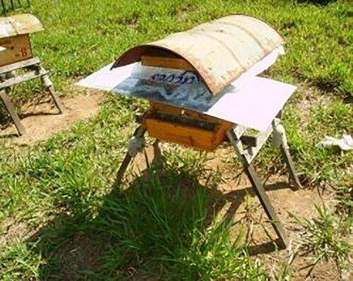
Figure 2. Pollen collection by beekeepers.

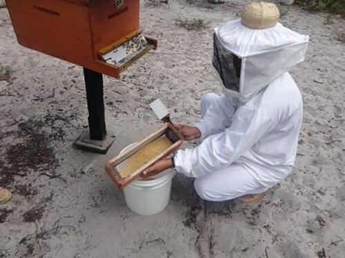
Figure 3. Conditions to be avoided in the apiary and surrounding area.

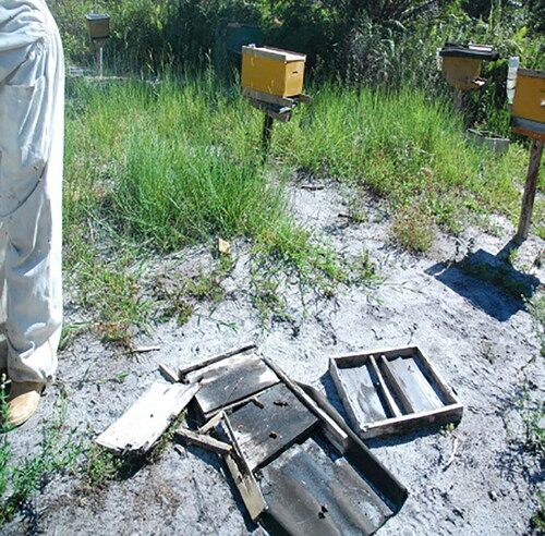
Figure 4. Bad conditions of the hives and packaging containers; hives on the ground are subject to rot and termite attack.

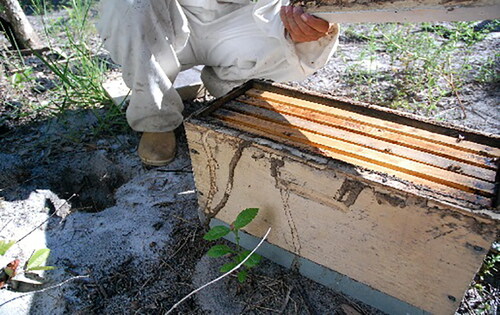
Figure 5. Damp compressed pollen.

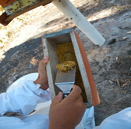
Figure 6. Processing “fresh” bee pollen; first screening.

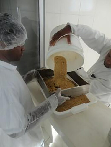
Figure 7. Example of a warehouse for bee pollen production in Brazil. This is one of the largest in Latin America, located in the state of Bahia, northeast Brazil. The main source of pollen is the coconut palm, achieving high standards of excellence and quality of the product: (a) Dehydration room 40 °C; (b) distribution trays; (c) aeration of the dehydrated product room.

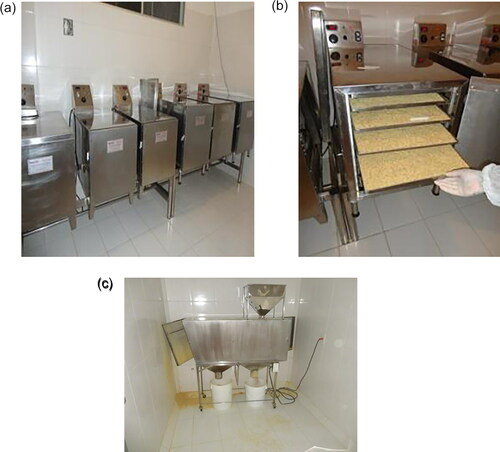
Figure 8. The proposed standard method for detecting unknown pollen loads. The processing chain finishes with an authentication output.

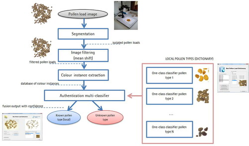
Figure 9. The computer vision system needs inexpensive hardware such as a camera and a stand to control illumination.

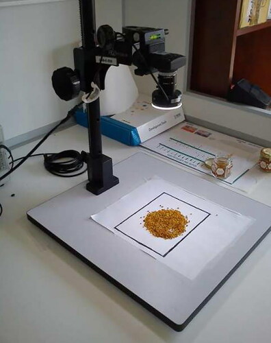
Figure 10. Different images of pollen load samples which were taken with our vision system. Left and central images belong to known pollen types (Rubus, Cistus ladanifer, Quercus ilex, and Echium, respectively). Right images are non-local samples and must be rejected by the system.

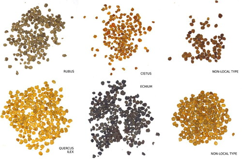
Figure 11. Original image and resulting images after applying the mean shift algorithm (varying spatial bandwidth $h_s$ to 7, 15, and 30, respectively).

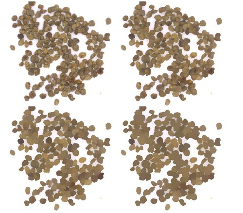
Table 1. Description of the three independent datasets used to train, test the classifiers, and validate the one-class multi-classifier.

Dataset name	Total size	Pollen types instances	Outlier instances
Training	400	400	0
Test	800	400	400
Validation	1946	1016	930

Table 2. Evaluation measures obtained by the one-class kNN classifiers for each of the four pollen types.

Rubus			Echium
FN rate	FP rate	F-measure	FN rate	FP rate	F-measure
0.05	0	0.9744	0.09	0	0.9529
Cistus ladanifer			Quercus Ilex
FN rate	FP rate	F-measure	FN rate	FP-rate	F-measure
0.06	0	0.9691	0.01	0.0028	0.9851

Lower values mean better performance.

Table 3. Evaluation measures of the final multi-classifier.

$\mathit{kNN}$ multi-classifier model	Accuracy (%)	FN rate	FP rate
0% rejected during training	92.5488	0.0108	0.1161
10% rejected during training	94.6043	0.0935	0.0167

Two cases are listed; considering 0%, and considering 10% of data as outliers when training the one-class classifiers. FN and FP rates are calculated taking all the known pollen types as the positive class and the outliers as the negative.

Table 4. Confusion matrix of the multi-classification system formed by the four one-class kNN classifiers (one for each pollen type).

	Predicted pollen type
Real pollen type		Rubus	Echium	Cistus	Quercus	Outlier	Total
	Rubus	248	0	0	0	33	281
	Echium	0	357	0	0	43	400
	Cistus	0	0	275	1	10	286
	Quercus	0	0	0	48	1	49
	Outlier	4	0	5	8	913	930
		Total	252	357	280	57	1000	1946

10% of the training data were rejected as outliers during the training phase of the one-class classifier.

Figure 12. Pollen load samples separated by an expert to train the system.

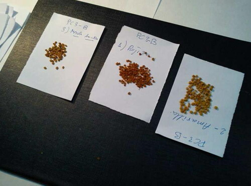
Figure 13. Screenshot of the prototype pollen dictionary. The ambiguity discovery algorithm checks if there is an existing pollen type having identical features compared to the new sample.

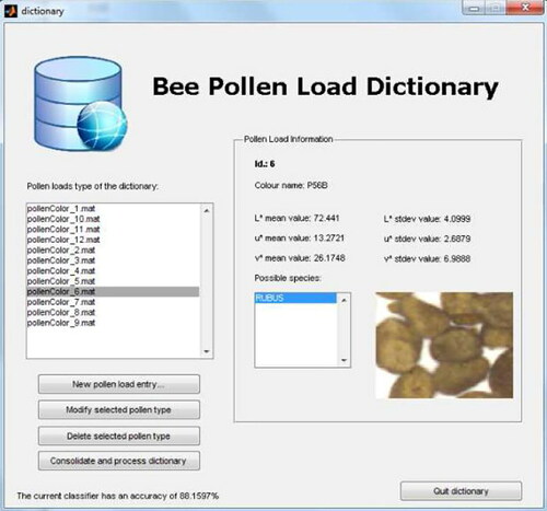
Figure 14. (a and b). Two screenshots of the prototype software detecting a local pollen type in the pollen load images.

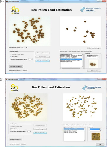
Figure 15. Flowchart of image analysis.

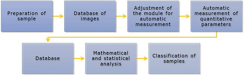
Figure 16. Evaluation of corbicula size characteristics.

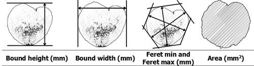
Figure 17. Evaluation of corbicula shape.

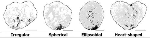
Figure 18. Evaluation of corbicula heart shape.

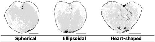
Figure 19. Evaluation of corbicula cutout depth.

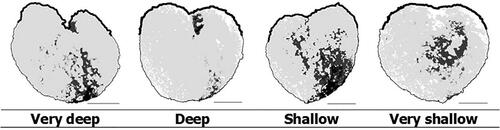
Figure 20. Evaluation of corbicula surface.

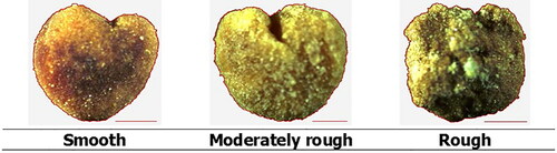
Figure 21. Flow chart of the descriptors list structure.

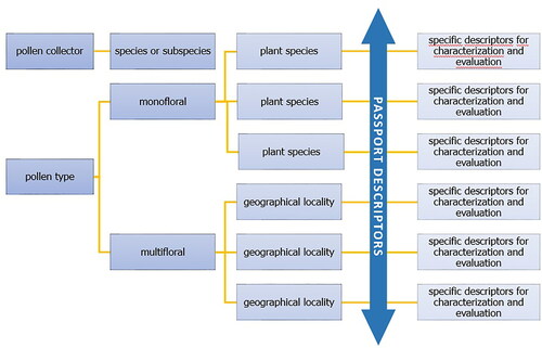
Figure 22. Descriptor structure.

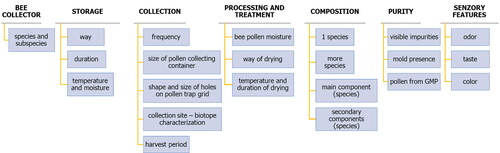
Table 5. Descriptor for quantitative character – principle of completeness.

Corbicula – height (mm)
1	Very small	< 2.30
3	Small	2.30 − 2.79
5	Medium	2.79 − 3.40
7	High	3.40 − 3.89
9	Very high	3.89 and more

Table 6. Structure of open and closed intervals in descriptor grades.

Corbicula – height (mm)
1	Very small	< 2.30	(0;2.30)
3	Small	2.30–2.79	(2.30;2.79)
5	Medium	2.79–3.40	(2.79;3.40)
7	High	3.40–3.89	(3.40;3.89)
9	Very high	3.89 and more	(3.89;∞)

Figure 23. Visual representation of the line for the limit points x_min = 1.81; x_max = 4.26 and the coordinate “x₄” to the point “y₄.”

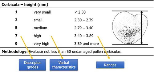
Figure 24. Flowchart of the passport data structure.

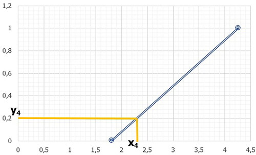
Table 7. Calculated value of variable “x.”

x1	x2	x3	x4	x5	x6	x7	x8	x9	x10	x11	x12	x13	x14	x15	x16	x17	x18	x19
1.93	2.06	2.18	2.30	2.42	2.55	2.67	2.79	2.91	3.04	3.16	3.28	3.40	3.53	3.65	3.77	3.89	4.02	4.14

Table 8. Determination of limit points in ranges for five descriptor levels.

x1	x2	x3	x4	x5	x6	x7	x8	x9	x10	x11	x12	x13	x14	x15	x16	x17	x18	x19
1.93	2.06	2.18	2.30	2.42	2.55	2.67	2.79	2.91	3.04	3.16	3.28	3.40	3.53	3.65	3.77	3.89	4.02	4.14

Table 9. Ranges of 5 descriptor levels for height.

Grade	Verbal characteristics	Intervals
1	Very small	< 2.30
3	Small	2.30–2.79
5	Medium	2.79–3.40
7	High	3.40–3.89
9	Very high	3.89 and more

Table 10. Descriptor for qualitative character – structure of grades.

Corbicula – heart shape
1	Elliptical
2	Spherical
3	Heart-shaped
9	Other

Table 11. Descriptor for qualitative character – structure of grades in the case of ordinal scale.

Corbicula – cutout depth
1	Very deep
3	Deep
7	Shallow
9	Very shallow

Table 12. Structure of alternative character.

Corbicula – presence of visible impurities
1	Absent
9	Present

Figure 25. Polarity in verbal description.

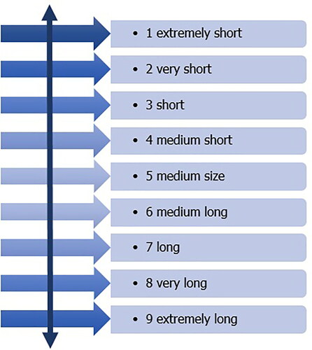
Table 13. Complete descriptor with methodology and pictures.

Grade	Verbal characteristics	Figures
3	Smooth	3	5	7
5	Moderately rough
7	Rough
Methodology: Evaluate not less than 50 undamaged pollen corbiculas.

Table 14. Descriptor for characteristic – corbicula – height (mm).

Grade	Verbal characteristics	Range	Figure
1	Very low
3	Low
5	Moderately high
7	High
9	Very high
Methodology: Evaluate at least 50 undamaged corbiculae, to two decimal places. The Figure shows the height (in the direction of axis y) of a bounded object.

Table 15. Descriptor for characteristic – corbicula – width (mm).

Grade	Verbal characteristics	Range	Figure
1	Very narrow
3	Narrow
5	Moderately wide
7	Wide
9	Very wide
Methodology: Evaluate at least 50 undamaged corbiculae, to two decimal places. The Figure shows the width (in the direction of axis x) of a bounded object.

Table 16. Descriptor for characteristic – corbicula – Feret maximum (mm).

Grade	Verbal characteristics	Range	Figure
1	Very small
3	Small
5	Medium
7	Large
9	Very large
Methodology: Evaluate at least 50 undamaged corbiculae.

Table 17. Descriptor for characteristic – corbicula – Feret minimum (mm).

Grade	Verbal characteristics	Range	Figure
1	Very small
3	Small
5	Medium
7	Large
9	Very large
Methodology: Evaluate at least 50 undamaged corbiculae.

Table 18. Descriptor for characteristic – corbicula – shape index (width/height).

Grade	Verbal characteristics	Range
3	ellipsoidal	<0.9
5	spherical	0.9–1.2
7	heart shaped	1.2 and more
Methodology: Evaluate at least 50 undamaged corbiculae.

Table 19. Descriptor for characteristic – corbicula – symmetry (Feret min/Feret max).

Grade	Verbal characteristics	Range
1	Unsymmetrical	0 − 0.81
9	Symmetrical	0.81 − 1
Methodology: Evaluate at least 50 undamaged corbiculae.

Table 20. Descriptor for characteristic – corbicula – area (mm²).

Grade	Verbal characteristics	Range	Figure
1	Very small
3	Small
5	Medium
7	Large
9	Very large
Methodology: Evaluate at least 50 undamaged corbiculae, to two decimal places. The area is determined by the boundaries of the object by distinguishing the limit color of the object from the background.

Table 21. Descriptor for characteristic – corbicula – weight (mg).

Grade	Verbal characteristics	Range
1	Very small
3	Small
5	Medium
7	Large
9	Very large
Methodology: Evaluate at least 50 undamaged corbiculae.

Table 22. Descriptor for characteristic – corbicula – texture.

Grade	Verbal characteristics	Figures
3	Smooth	3	5	7
5	Moderately rough
7	Rough
Methodology: Evaluate not less than 50 undamaged pollen corbiculas.

Table 23. Descriptor for characteristic – corbicula – shape.

Grade	Verbal characteristics	Figures
1	Irregular
2	Spherical
3	Ellipsoidal
4	Heart shaped
9	Other	1	2	3	4
Methodology: Evaluate not less than 50 undamaged pollen corbiculas

Table 24. Descriptor for characteristic – corbicula – heart shape.

Grade	Verbal characteristics	Figures
1	Ellipsoidal	1	2	3
2	Spherical
3	Heart shaped
4	Other
Methodology: Evaluate not less than 50 undamaged pollen corbiculas.

Table 25. Descriptor for characteristic – corbicula – cutout depth.

Grade	Verbal characteristics	Figures
1	Very shallow
3	Shallow
7	Deep
9	Very deep
		1	3	7	9
Methodology: Evaluate not less than 50 undamaged pollen corbiculas.

Table 26. Evaluation of corbicular color (Nôžková, Brindza et al., 2010).

Sample no.	Color (Visual assessment)	Color group name (RHS)	Color (RHS)
2	brownish yellow	gray-yellow	162 A
5	grayish green	gray-green	194 A
66	brown brick	gray-orange	165 B
80	lemon yellow	yellow	8 A
81	brownish yellow	gray-yellow	162 A
90	brownish yellow	gray-yellow	162 A
98	brownish yellow	gray-yellow	162 A
99	brownish yellow	gray-yellow	162 A
100	carrot orange	orange	24 A
113	brownish yellow	gray-orange	164 B

Table 27. Descriptor for characteristic – corbicula -color.

Grade	Verbal characteristics
1	Black
2	Purple
3	Brown
4	Green
5	Orange
6	Yellow
7
8
9	Other
Figures
2 purple hue
3 brown hue
4 green hue
5 orange hue
6 yellow hue
Methodology: Visual assessment: the most frequent corbicula color is taken into account and the corbicula is assigned its respective classification grade. Evaluation using RHS: the methodological rules set out in this classification system are observed. After determining the color of the sample, the respective code (e.g., 164B) is recorded.

Figure 26. Diagrams showing the structure of a pollen grain in optical section (Sawyer, 1981).

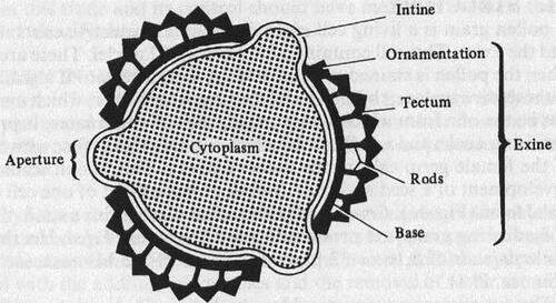
Figure 27. Diagrams showing details of pollen grain walls (Sawyer, 1981).

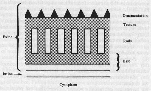
Figure 28. Diagrams illustrating the morphological regions of a pollen grain and pollen grain apertures: (a) equatorial view; (b) polar view (Sawyer, 1981).

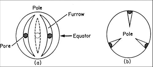
Table 28. Diagnostic pollen grain features used for identification (Vorwohl, 1990).

1.	Length and breadth	1	<10 µm
		2	10–15 µm
		3	15–20 µm
		4	20–25 µm
		5	25–30 µm
		6	30–35 µm
		7	35–40 µm
		8	40–50 µm
		9	>50 µm
2.	Aperture number	1
		2
		3
		4
		5
		6
		7
		8	>7
		9	Absent or not clear
3.	Aperture type	1	Pore
		2	Colpa
		3	Heterocolpa
		4	Syncolpate
		5	Heterocolporate
4.	Exine Sculpture	1	Psilate, Faveolate, Fossulate
		2	Scabrate, Verrucate, Gennuate
		3	Echinate
		4	Clavate, Bacculate
		5	Rugulate, Striate
		6	Reticulate
		7	Fenestrate
5	Aggregation	1	1
		2	2
		3	3
		4	4
		5	5
		6	6
		7	7
		8	>7

Figure 29. Photos to illustrate the variety of colors of pollen loads of different species of plants: (a) gray – Vicia faba; (b) lemon yellow – Brassica napus; (c) dark gray – Papaver rhoeas; (d) blue – Phacelia tanacetifolia; (e) mixed yellow pollen – mixed pollen from fruit trees (Prunus, Pyrus, Malus) and bright orange – Taraxacum officinale.

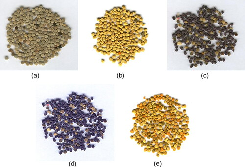
Figure 30. Typical (normal) pollen grains (scanning electron microscopy): (a) Aesculus hippocastanum; and (b) Vicia faba.

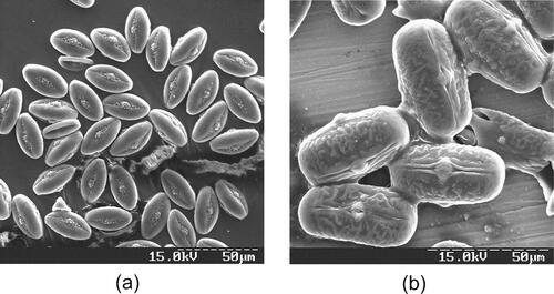
Figure 31. Pollen grains with changed morphological structures (scanning electron microscopy): (a) Phacelia tanacetifolia; (b) Taraxacum officinale; and (c) Scilla bifolia.

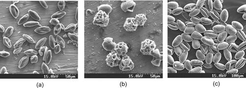
Figure 32. Separation of bee pollen by color pellets from a sample that include different floral origin pollens.

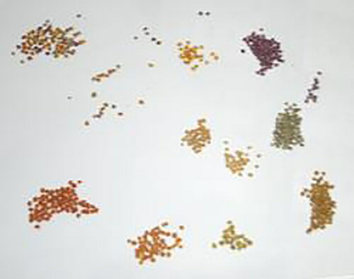
Figure 33. Basic flavonoid structure in order to show a better understanding of the explanation of the UV spectra related to the position of the substitution in the molecule (From Campos & Markham, 2007. Reproduced with permission).

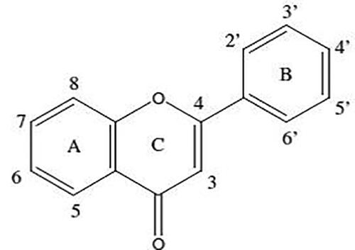
Figure 34. Examples of the more common UV- spectra found in bee pollens: (a) apigenin; (b) apigenin-7-O-derivative; (c) luteolin; (d) kaempferol-3-O-derivative; (e) quercitin-3-O-derivative; (f) isorhamnetin-3-O-derivative; (g) chalcone.

Figure 35. Fingerprint of Eucalyptus globulus obtained with a pollen pellet (100% pure) and a mixture of bee pollen with about 60% of Eucalyptus globulus pollen pellets.

Table 29. Amplitude of the Wavelengths in Band I of flavones and flavonols UV spectra.

Flavonoid type	λ (nm)
Flavones	304–350
Flavonols (OH-3 derivative)	328–357
Flavonol (OH-3 free)	352–385

Table 30. Wavelengths of Band I in UV spectra of flavonols with a different pattern of oxygenation in B-ring.

	Oxigenation pattern
Flavonols	Ring-A and C	Ring-B	λmax. (nm)
Galangin	3,5,7	–	359
kampferol	3,5,7	4′	367
Quercetin	3,5,7	3′, 4′	370
Myricetin	3,5,7	3′, 4′, 5′	374

Table 31. Wavelengths of Band II in UV spectra of flavones with oxygenation only in A-ring.

Flavone	Oxygenation pattern of A-ring	λmax. (nm)
Flavone		250
5-hydroxiflavone	5	268
7-hydroxiflavone	7	252
5,7-di-hydroxiflavone	5.7	268
Baicalein	5,6,7	274
Norwogonin	5,7,8	281

Table 32. Model of chemical structures of subclasses or representative molecule of subclasses of non-flavonoids phenolic compounds.

Subclass	Model of chemical structure or model of representative molecule	Name
Lignans		virolin
Lignins		pinoresinol
Phenolic acids		hydroxycinnamic acids
		hydroxybenzoic acids
Coumarins		coumarin
Stilbenes		resveratrol
Tannins		gallotannin

Table 33. Model of chemical structures of flavonoids.

Subclass	Model of chemical structure
Chalcones
Aurones
Flavanols
Flavonols
Flavones
Flavanones
Isoflavones
Antocyanins

Figure 36. General formula of flavonoids.

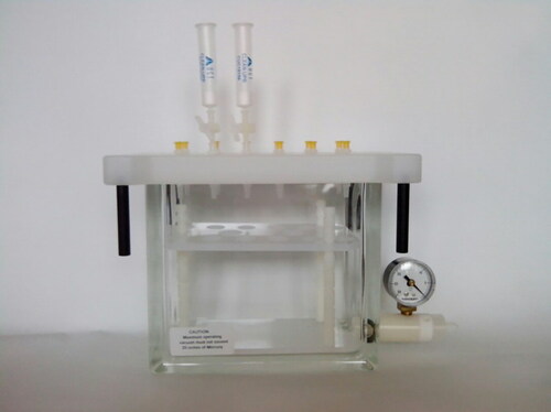
Table 34. Some publications on LC and LC/MS analysis of polyphenolic compounds from bee pollen samples.

Compounds	Method	Stationary phase	Mobile phase		t (°C)	Flow rate (mL/min)	λ (nm)	References
			A	B
Flavonoids	HPLC-PAD	C18 11.9 cm × 0.4 cm, 5 µm	Orthophosphoric acid pH 2.5	Acetonitrile	24	0.8	220-400	Campos et al. (1997)
Flavonoids (aglycons)	HPLC-DAD	C18 4.6 mm × 250 mm, 10 µm	Orthophosphoric acid pH 2.6	Methanol		2	278-282 278-350	Serra-Bonvehí et al. (2001)
Phenolic acids, flavonoids	Nano-LC-UV	C18 100 µm I.D. × 10 cm	0.5% formic acid	Methanol		500 nl/min	200, 280	Fanali et al. (2013)
Anthocyanins	HPLC-DAD-ESI-MS/MS	C18 150 mm × 4.6 mm, 5 µm	0.1% trifluoracetic acid	Acetonitrile	35	0.5	520	Di Paola-Naranjo et al. (2004)
Flavonoids	HPLC-PAD-ESI-MS/MS	C18 250 mm × 4 mm, 5 µm	1% formic acid	Methanol		1	350, 520	Ferreres et al. (2010)
Flavonoids, hydroxycinnamic acid amide derivatives	HPLC-PAD-ESI-MS/MS	C18 250 mm × 4.6 mm, 5 µm	0.1% acetic acid	Methanol	28	0.5	270, 350	Negri et al. (2011)
Flavonoid aglycones	HPLC-DAD-APCI/MS	C8 150 mm × 4.6 mm, 5 µm	0.1% formic acid in 5% acetonitrile	Acetonitrile	30	1	258	Lv et al. (2015)

Figure 37. Solid phase extraction.

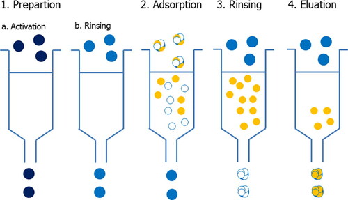
Table 37. International data on the protein content (% D.M) of bee pollen.

Crude protein content (% D.M)
Type of samples	Number of samples	Values	References
Multifloral	21	21.0–29.3	Herbert & Shimanuki, 1978
Multifloral	20	12.6–18.2	Serra-Bonvehí & Escolá Jordá, 1997
Monofloral	194	9.2–37.4	Somerville, 2001
Multifloral	15	9.8–16.5	Villanueva et al., 2002
Monofloral	29	13.6–31.9	Andrada & Telleria, 2005
Multifloral	10	21 ± 4*	Almeida-Muradian et al., 2005
Multifloral	6 batches	23.59**	Melo et al., 2005
Monofloral	123	13.0–24.5	Szczêsna, 2006a
Multifloral (Poland)	13	15.8–24.1	Szczêsna, 2006b
Multifloral (Korea)	9	17.6–24.5	Szczêsna, 2006b
Multifloral (China)	5	17.8–26.1	Szczêsna, 2006b
Monofloral	42	6.3–26.3	Forcone et al., 2011
Multifloral	154	12.2–27.0	Martins et al., 2011
Multifloral	14	18.4–22.4	Balkanska & Ignatova, 2012
Multifloral	7	15.2–28.5	Stanciu et al., 2012
Monofloral	12	14.2–28.9	Yang et al., 2014
Multifloral	7 batches	23.38 ± 1.24*	(Arruda et al., 2013)
Multifloral	106	13.65–26.5	(Liolios et al., 2014)
Monofloral	58	9.7–30.11	(Liolios et al., 2014)

* Average and standard deviation.

** Average.

Table 35. Mass spectral data of compounds detected in extracts of bee pollen.

No	[M + H]^+, m/z	[M-H]^-, m/z	MS/MS positive ion mode	MS/MS negative ion mode	Proposed identification	References
1	685.0				Rosmarinic acid dihexoside derivative	Negri et al. (2011)
2	627.2		481.0, 319.0		Myricetin-3-O-rhamnosyl-glucoside	Negri et al. (2011)
3	435.0		303.0		Quercetin-3-O-arabinoside	Negri et al. (2011)
4	641.2		479.0, 317.0		Isorhamnetin-3-O-diglucoside	Negri et al. (2011)
5	595.0		449.0, 287.0		Kaempferol-3-O- rhamnosyl-glucoside	Negri et al. (2011)
6	771.2		625.1, 479.1, 317.1		Isorhamnetin-3-O- (2′',3′’-dirhamnosyl)glucoside	Negri et al. (2011)
7	611.1		303.1		Rutin	Negri et al. (2011)
8	625.2		479.0, 317.0		Isorhamnetin-3-O- rhamnosyl-glucoside	Negri et al. (2011)
9	449.0		287.0		Kaempferol-3-O-glucoside	Negri et al. (2011)
10	641.2		495.0, 333.0		Patuletin-3-O- rhamnosylglucoside	Negri et al. (2011)
11	449.2		303.1 (100%)		Quercitrin	Negri et al. (2011)
12	381.4		261.0, 235.2, 147.2		Chalcone	Negri et al. (2011)
13	761.3		615.3, 381.1, 287.0		Kaempferol-7-O-rhamnosyl-3-O-galloyl glucuronide	Negri et al. (2011)
14	584.3		438.2, 420.2		N’ ,N’’ ,N’’’-tris-p-coumaroylspermidine	Negri et al. (2011)
15	674.3		498.2 , 480.3		N’ ,N’’ ,N’’’-tris-p-feruloylspermidine	Negri et al. (2011)
16	465		303		Delphinidin-3-O-glucoside	Di Paola-Naranjo et al. (2004)
17	611		303, 465		Delphinidin-3-O-rutinoside	Di Paola-Naranjo et al. (2004)
18	449		287		Cyanidin-3-O-glucoside	Di Paola-Naranjo et al. (2004)
19	595		287, 449		Cyanidin-3-O-rutinoside	Di Paola-Naranjo et al. (2004)
20	479		317		Petunidin-3-O-glucoside	Di Paola-Naranjo et al. (2004)
21	625		317, 479		Petunidin-3-O-rutinoside	Di Paola-Naranjo et al. (2004)
22	609		301, 463		Peonidin-3-O-rutinoside	Di Paola-Naranjo et al. (2004)
23	639		331, 493		Malvidin-3-O-rutinoside	Di Paola-Naranjo et al. (2004)
24	535		287, 449		Cyanidin-3-(6′’-malonylglucoside)	Di Paola-Naranjo et al. (2004)
25		625		463, 445, 300	Quercetin-3- sophoroside	Ferreres et al. (2010)
26		623		315	Isorhamnerin-3- rutinoside	Ferreres et al. (2010)
27		609		463, 445, 300	Quercetin-3- neohesperidoside	Ferreres et al. (2010)
28		609		447, 429, 285	Kaempferol-3- sophoroside	Ferreres et al. (2010)
29		739		593, 575, 284	Kaempferol-3-(4- rhamnosyl)- neohesperidoside	Ferreres et al. (2010)
30		593		447, 429, 284	Kaempferol- 3- neohesperidoside	Ferreres et al. (2010)
31		635		593, 489, 471, 284	Kaempferol-3-(acetyl)- neohesperidoside	Ferreres et al. (2010)
32		739		593, 285	Kaempferol-3- neohesperidosyl- 7- rhamnoside	Ferreres et al. (2010)
33		447		285	Kaempferol-3- glucoside	Ferreres et al. (2010)
34		593		285	Kaempferol-3- rutinoside	Ferreres et al. (2010)
35		635		593, 489, 471, 284	Kaempferol- 3- (acetyl)- neohesperidoside isomer	Ferreres et al. (2010)

Table 36. Primer Sequences with indexes SA501 – SB712 (adapted from Kozich et al., 2013).

Forward
Name	Sequence
SA501	AATGATACGGCGACCACCGAGATCTACAC ATCGTACG CCTGGTGCTG GT ATGCGATACTTGGTGTGAAT
SA502	AATGATACGGCGACCACCGAGATCTACAC ACTATCTG CCTGGTGCTG GT ATGCGATACTTGGTGTGAAT
SA503	AATGATACGGCGACCACCGAGATCTACAC TAGCGAGT CCTGGTGCTG GT ATGCGATACTTGGTGTGAAT
SA504	AATGATACGGCGACCACCGAGATCTACAC CTGCGTGT CCTGGTGCTG GT ATGCGATACTTGGTGTGAAT
SA505	AATGATACGGCGACCACCGAGATCTACAC TCATCGAG CCTGGTGCTG GT ATGCGATACTTGGTGTGAAT
SA506	AATGATACGGCGACCACCGAGATCTACAC CGTGAGTG CCTGGTGCTG GT ATGCGATACTTGGTGTGAAT
SA507	AATGATACGGCGACCACCGAGATCTACAC GGATATCT CCTGGTGCTG GT ATGCGATACTTGGTGTGAAT
SA508	AATGATACGGCGACCACCGAGATCTACAC GACACCGT CCTGGTGCTG GT ATGCGATACTTGGTGTGAAT
SB501	AATGATACGGCGACCACCGAGATCTACAC CTACTATA CCTGGTGCTG GT ATGCGATACTTGGTGTGAAT
SB502	AATGATACGGCGACCACCGAGATCTACAC CGTTACTA CCTGGTGCTG GT ATGCGATACTTGGTGTGAAT
SB503	AATGATACGGCGACCACCGAGATCTACAC AGAGTCAC CCTGGTGCTG GT ATGCGATACTTGGTGTGAAT
SB504	AATGATACGGCGACCACCGAGATCTACAC TACGAGAC CCTGGTGCTG GT ATGCGATACTTGGTGTGAAT
SB505	AATGATACGGCGACCACCGAGATCTACAC ACGTCTCG CCTGGTGCTG GT ATGCGATACTTGGTGTGAAT
SB506	AATGATACGGCGACCACCGAGATCTACAC TCGACGAG CCTGGTGCTG GT ATGCGATACTTGGTGTGAAT
SB507	AATGATACGGCGACCACCGAGATCTACAC GATCGTGT CCTGGTGCTG GT ATGCGATACTTGGTGTGAAT
SB508	AATGATACGGCGACCACCGAGATCTACAC GTCAGATA CCTGGTGCTG GT ATGCGATACTTGGTGTGAAT
Reverse
Name	Sequence
SA701	CAAGCAGAAGACGGCATACGAGAT AACTCTCG AGTCAGTCAG CC TCCTCCGCTTATTGATATGC
SA702	CAAGCAGAAGACGGCATACGAGAT ACTATGTC AGTCAGTCAG CC TCCTCCGCTTATTGATATGC
SA703	CAAGCAGAAGACGGCATACGAGAT AGTAGCGT AGTCAGTCAG CC TCCTCCGCTTATTGATATGC
SA704	CAAGCAGAAGACGGCATACGAGAT CAGTGAGT AGTCAGTCAG CC TCCTCCGCTTATTGATATGC
SA705	CAAGCAGAAGACGGCATACGAGAT CGTACTCA AGTCAGTCAG CC TCCTCCGCTTATTGATATGC
SA706	CAAGCAGAAGACGGCATACGAGAT CTACGCAG AGTCAGTCAG CC TCCTCCGCTTATTGATATGC
SA707	CAAGCAGAAGACGGCATACGAGAT GGAGACTA AGTCAGTCAG CC TCCTCCGCTTATTGATATGC
SA708	CAAGCAGAAGACGGCATACGAGAT GTCGCTCG AGTCAGTCAG CC TCCTCCGCTTATTGATATGC
SA709	CAAGCAGAAGACGGCATACGAGAT GTCGTAGT AGTCAGTCAG CC TCCTCCGCTTATTGATATGC
SA710	CAAGCAGAAGACGGCATACGAGAT TAGCAGAC AGTCAGTCAG CC TCCTCCGCTTATTGATATGC
SA711	CAAGCAGAAGACGGCATACGAGAT TCATAGAC AGTCAGTCAG CC TCCTCCGCTTATTGATATGC
SA712	CAAGCAGAAGACGGCATACGAGAT TCGCTATA AGTCAGTCAG CC TCCTCCGCTTATTGATATGC
SB701	CAAGCAGAAGACGGCATACGAGAT AAGTCGAG AGTCAGTCAG CC TCCTCCGCTTATTGATATGC
SB702	CAAGCAGAAGACGGCATACGAGAT ATACTTCG AGTCAGTCAG CC TCCTCCGCTTATTGATATGC
SB703	CAAGCAGAAGACGGCATACGAGAT AGCTGCTA AGTCAGTCAG CC TCCTCCGCTTATTGATATGC
SB704	CAAGCAGAAGACGGCATACGAGAT CATAGAGA AGTCAGTCAG CC TCCTCCGCTTATTGATATGC
SB705	CAAGCAGAAGACGGCATACGAGAT CGTAGATC AGTCAGTCAG CC TCCTCCGCTTATTGATATGC
SB706	CAAGCAGAAGACGGCATACGAGAT CTCGTTAC AGTCAGTCAG CC TCCTCCGCTTATTGATATGC
SB707	CAAGCAGAAGACGGCATACGAGAT GCGCACGT AGTCAGTCAG CC TCCTCCGCTTATTGATATGC
SB708	CAAGCAGAAGACGGCATACGAGAT GGTACTAT AGTCAGTCAG CC TCCTCCGCTTATTGATATGC
SB709	CAAGCAGAAGACGGCATACGAGAT GTATACGC AGTCAGTCAG CC TCCTCCGCTTATTGATATGC
SB710	CAAGCAGAAGACGGCATACGAGAT TACGAGCA AGTCAGTCAG CC TCCTCCGCTTATTGATATGC
SB711	CAAGCAGAAGACGGCATACGAGAT TCAGCGTT AGTCAGTCAG CC TCCTCCGCTTATTGATATGC
SB712	CAAGCAGAAGACGGCATACGAGAT TCGCTACG AGTCAGTCAG CC TCCTCCGCTTATTGATATGC
Index and Read
Name	Sequence
Read1	CCTGGTGCTG GT ATGCGATACTTGGTGTGAAT
Read2	AGTCAGTCAG CC TCCTCCGCTTATTGATATGC
Index	GCATATCAATAAGCGGAGGA GG CTGACTGACT

Index sequences indicated in bold.

Figure 38. Base peak chromatograms of (a) cherry wine and (b) Cabernet Sauvignon-Central Serbia in positive ion mode. (Pantelić et al., 2014).

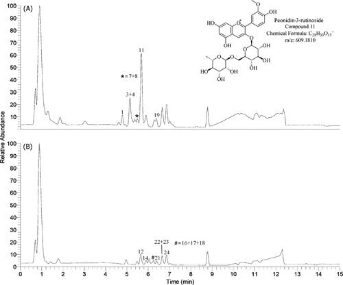
Figure 39. Extracted ion chromatograms and MS/MS spectra of cyanidin-3-rutinoside (Pantelić et al., 2014).

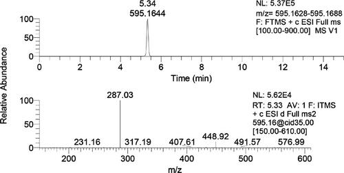
Table 39. Protein content (%) using different distillation times.

Distillation time (min)	Protein content (%) n = 5
4	20.48 (± 0.07)^a
3	20.29 (± 0.25)^a
2	20.41 (± 0.04)^a

Table 40. Protein content (%) analyzing different quantities of pollen.

Pollen quantity (g)	Protein content (%) n = 5
0.5	19.12 (± 0.16)^b
1	20.59 (± 0.03)^a
2	20.64 (± 0.06)^a

Different letter shows statistically significant changes (Duncan’s multiple range test, α = 0.005).

Table 38. Determination of the protein content (%) using different volumes of the H₃BO₃ solution.

Volume of H3BO3 (ml)	Protein content (%) n = 5
30	20.49 (± 0.07)^a
40	20.44 (± 0.06)^a

Analysis performed under the same conditions except the volume of the H₃BO₃ solution used.

Table 43. Total lipid content (%) in pollen samples, by using different elution times (3 h, 5 h, 7 h).

Elution time (h)	Total lipid content % (n = 5)
3	2.56 (±0.080)^a
5	2.95(±0.040)^b
7	2.96 (±0.025)^b

The pollen amount was 2 g and the petroleum ether served as solvent. Different Latin letter indicates statistically significant differences, according to Duncan’s multiple range test (a = 0.05).

Figure 40. (a) Extracted ion chromatograms of phenolic glyceride derivatives with their retention times and accurate masses; (b and c) mass spectra of two phenolic glyceride derivatives with the same accurate masses, m/z 413 (Ristivojević et al. 2014).

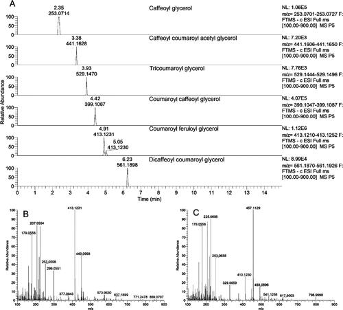
Figure 41. Planning scheme for samples and the corresponding index-combinations. Roman numbers indicate PCR plate numbers, bold Arabian numbers on 96 well plates indicate normalization plate number.

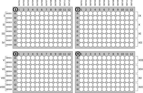
Table 41. International data on the lipid content (% DM) of bee pollen.

Crude lipid content (%D.M)
Type of samples	Number of samples	Values	References
Multifloral	21	4.0–5.5	(Herbert & Shimanuki, 1978)
Multifloral	3	2.0–18.0	(Echigo et al., 1986)
Multifloral	20	4.8–7.1	(Serra-Bonvehí & Escolá Jordá, 1997)
Monofloral	172	0–11.2	(Somerville, 2001)
Multifloral	15	3.6–8.9	(Villanueva et al., 2002)
Multifloral	10	7 ± 2*	(Almeida-Muradian et al., 2005)
Multifloral	6 batches	4.97**	(Melo et al., 2005)
Multifloral (Korea)	9	3.3–9.8	(Szczêsna, 2006a)
Multifloral (China)	5	3.5–8.8	(Szczêsna, 2006b)
Multifloral (Poland)	13	6.74–10.99	(Szczêsna, 2006c)
Multifloral	154	4.0–13.3	(Martins et al., 2011)
Multifloral	7	4.3–5.0	(Stanciu et al., 2012)
Multifloral	14	6.3–8.7	(Balkanska & Ignatova, 2012)
Monofloral	12	0.6–6.5	(Yang et al., 2014)
Multifloral	7 batches	5.39 ± 0.60*	(Arruda et al., 2013)
Multifloral	99	1.15–6.97	(Liolios et al., 2014)
Monofloral	43	0.4–13.6	(Liolios et al., 2014)

*Average and standard deviation; ** Average.

Table 42. Total lipid content (%) by using different amount of pollen for the analysis.

Pollen amount (g)	Total lipid content % (n = 5)
1	2.24 (±0.113)^a
2	2.87 (±0.056)^b
3	2.83 (±0.098)^b

The elution time was equal (5 h) and the petroleum ether served as solvent. Different Latin letter indicates statistically significant differences, according to Duncan’s multiple range test (a = 0.05).

Table 44. Total lipid content (%) in pollen samples, by using different solvents (acetone, petroleum ether, hexane).

Solvent	Total lipid content % n = 5
Acetone	2.99 (±0.155)^a
Petroleum ether	2.91 (±0.084)^a
Hexane	2.9 (±0.268)^a

The pollen amount was 2 g and the elution time was 5 h.

Figure 42. Detailed workflow (schematic), suitable for laboratories with limited access to equipment for automated pipetting. Bold numbers indicated step number of Design 2 in Section 8.1.3.2.

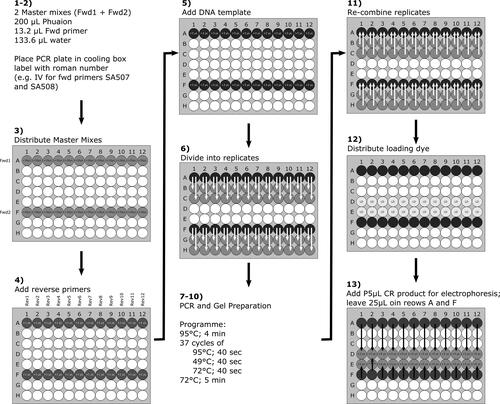
Figure 43. Crude protein content (% D.M) of bee pollen from selected botanical origins.

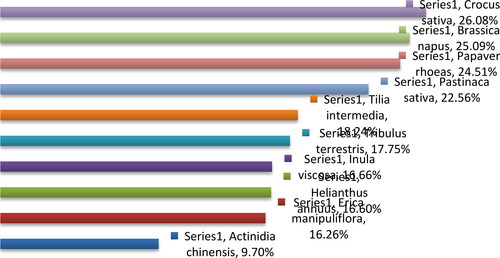
Figure 44. Protein content (% D.M) of mixed pollen samples harvested during the beekeeping season of 2011.

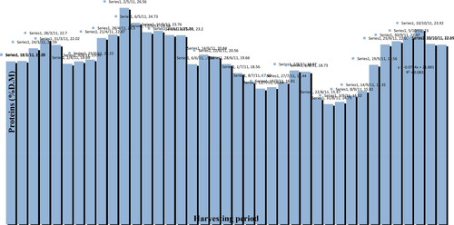
Figure 45. Crude lipid content (% D.M) of bee pollen from selected botanical origins.

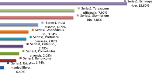
Figure 46. Lipid content (% D.M) of mixed pollen samples harvested during the beekeeping season of 2013.

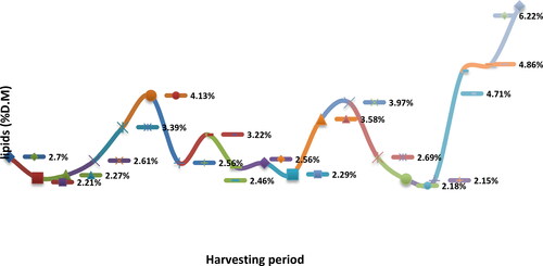
Figure 47. (a) Structure of PAs: Necinic acids are connected to the necine base by ester bond in position 1 and/or 7. Necinic acids can be connected to form a macrocyclic ester; (b) Example of PA free base and N-oxide macrocyclic esters (Hartmann & Witte, 1995).

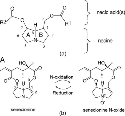
Table 45. Literature data on the carbohydrate content of bee pollen calculated as: 100 – (g fat + g protein + g ash + g water) (g/100 g DM).

Type of samples	Number of samples	Values	References
Monofloral (Aloe greatheadii var. davyana)	6	59.5 (±1.3)*	Human and Nicolson (2006)
Multiflora	22	67.7 (±2.6)* 61.2–70.6**	Feas et al. (2012)
Multifloral	8	69.68–84.25**	Nogueira et al. (2012)
Monoflora (Brasica napus L., Citrullus lanatus L., Camellia japonica L., Dendranthema indicum L., Fagopyrum esculentum L., Helianthus annus L., Nelumbo nucifera Gaertn., Papaver rhoeas L., Rosa rugosa, Schisandra chinensis, Vicia faba L., Zea mays L.)	12	59.43–77.82**	Yang et al. (2014)
Multifloral	–	13–55**	Bogdanov (2015)
Multifloral	26	64.42–81.84**	Kostić et al. (2015)

*Average and standard deviation; **min – max.

Table 46. Literature data on the content of sugars in bee pollen (g/100 g DM).

Type of samples/Country of origin	Number of samples	Sugars	Values	Method used References
Multiflora (with a predominance of Cistus landaniferus)/ Spain	20	Fructose	15.20–23.90*	GC-FID Serra-Bonvehí & Escolá Jordá (1997)
		Glucose	10.86–18.19*
		Saccharose	4.20–9.40*
		Maltose	0.79–3.20*
		F/G****	1.13–1.53*
Multifloral/Poland	95	Fructose	13.38–21.80*	GC-FID Szczęsna et al. (2002)
		Glucose	5.99–18.17*
		Saccharose	3.74–7.59*
		Maltose	0.96–3.32*
		F/G****	1.03–2.51*
Multifloral/ Poland, South Korea, China	27	Fructose	9.74–22.06*	HPLC-RID Szczęsna (2007)
		Glucose	8.45–20.06*
		Saccharose	1.13–4.84*
		Maltose	1.07–3.51*
		F/G****	1.02–1.63*
Multifloral/Israel, China, Romania, Spain	5	Fructose	15.9–19.9*	HPLEC-PAD Qian et al. (2008)
		Glucose	8.2–13.1*
		Saccharose	14.8–18.4*
		F/G****	1.33–1.66*
Multifloral/Romania	-***	Fructose	19.31**	HPLC-RID Bobis et al. (2010)
		Glucose	17.86**
		Saccharose	0.85**
		Maltose	0.64**
Multifloral/Brazil	154	Fructose	12.59–23.62*	HPLC-RID Martins et al. (2011)
		Glucose	6.99–21.85*
		F/G****	1.01–2.24
Multifloral/Romania	16	Fructose	8.44–15.39*	HPLC-RID Mărgăoan et al. (2012)*****
		Glucose	4.37–16.14**
		F/G****	0.78–1.44*
Monofloral (Cucurbita pepo Thunb, Phoenix dactylifera L., Helianthus annus L., Medicago sativa L., Brasica napus L.)/ Saudi Arabia	-***	Fructose	17.13–21.30*	HPLC-RID Taha (2015)
		Glucose	15.44–17.06*
		F/G****	1.07–1.25*

*min – max; **average; ***no information; ****fructose to glucose ratio; *****results for fresh pollen.

Table 47. Methods used to evaluate the vitamin content of bee pollen.

Method	Vitamins analyzed	Country	Reference	Vitamin content (mean)
Open column chromatography and microfluorimetric method	C, beta-carotene as provitamin A	Brazil	Almeida-Muradian et al., 2005	Absence of vitamin C and beta-carotene (dried bee pollen)
Open column chromatography and titrimetric method	E, C and beta-carotene as provitamin A	Brazil	Oliveira et al., 2009	13,5 µg/g (E); 56,3–198,9 µg/g (beta-carotene); 273,9–560,3 µg/g (C) (fresh bee pollen)
HPLC, open column chromatography and titrimetric method	E, C and beta-carotene as provitamin A	Brazil	Melo et al., 2009	114–340 µg/g (C); 16,27–38,64 µg/g (E); 3,14–77,88 µg/g (beta carotene) (dried bee pollen)
HPLC, open column chromatography and titrimetric method	E, C and beta-carotene as provitamin A	Brazil	Melo & Almeida-Muradian, 2010	14–119 ug/g (C); 19.43–37.19 µg/g (E); 5.95–99.27 µg/g (beta-carotene) (fresh bee pollen)
HPLC method with fluorescence detection.	B1, B2, B6 and PP	Brazil	Arruda et al., 2013a; Arruda et al., 2013b	0.64 mg/100 g (B1); 0.60 mg/100 g (B2); 12.18 mg/100 g (PP); 0.55 mg/100 g (B6)
HPLC and titrimetric method	E (alpha, beta, gamma and delta tocoperol), C (ascorbic acid) and provitamin A (alpha and beta-carotene)	Brazil	Sattler, 2013	60–797 µg/g (C); 0.57–11.7 mg/100g (E); 0–179.21 µg/g of beta-carotene; 0–828.43 µg/g of alpha-carotene
HPLC method with fluorescence detection.		Brazil	Souza, 2014	0.46–1.57 mg/100g (B1); 0.40–1.86 mg/100g (B2); 2.67–7.74 mg/100g (PP or B3);0.78–7.13 mg/100g (B6)

Table 48. Calibration curves obtained for echimidine, lycopsamine and intermedine.

Echimidine or Lycopsamine or Intermedine (µg/ml)	Echimidine (intensity)	Intermedine (intensity)	Lycopsamine (intensity)
0.02	2950	3130	3670
0.1	13660	15540	16200
0.5	63940	62050	71200
2	243800	200400	277000
Calibration curve*	y = 122755x + 686	y = 104410x + 1900	y = 138740x + 1143

* Weighted by 1/x.

Table 51. PAs which have not been previously reported from E. vulgare and E. cannabinum.

Compound name	RT (min)	Chemical formula	[M + H]^+ experimental	[M + H]^+ calculated	Error (mDa)
Echium vulgare
Curassavine-N-oxide*	1.54	C16H29NO5	316.2125	316.2124	0.1
Eupatorium cannabinum
Leptantine*	1.41	C15H27NO6	318.1922	318.1917	0.5
Amabiline*	1.48	C15H25NO4	284.1865	284.1862	0.3
Uplandicine*
	1.71	C17H27NO7	358.1868	358.1866	0.2

* Tentative identification.

Table 50. MS/MS fragment ions for PA-N-oxides from E. vulgare or E. cannabinum.

Pyrrolizidine alkaloid	[M + H]^+	MS/MS fragment ions
Echium vulgare
Echimidine-N-oxide	414.2126	396.2029, 352.1764, 338.1608, 254.1403, 220.1350, 120.0817
Acetylechimidine-N-oxide	456.2234	438.2131, 396.2025, 338.1610, 254.1393, 220.1339
Echivulgarine-N-oxide	496.3402	478.2448, 396.2030, 338.1613, 254.1397, 220.1341, 120.0816
Vulgarine-N-oxide	414.2133	396.2021, 314.1612, 256.1189, 172.0976, 138.0923, 136.0764
Acetylvulgarine-N-oxide	456.2243	438.2132, 356.1714, 298.1295, 214.1081, 180.1030, 120.0818
Eupatorium cannabinum
Lycopsamine/Intermedine-N-oxide	316.1756	172.0973, 155.0947, 138.0917, 111.0684

Figure 48. (a and b) Structure of a flower of E. vulgare.

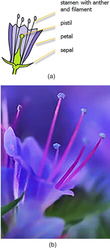
Figure 49. An E. vulgare plant bagged with a net and supported by a metal structure.

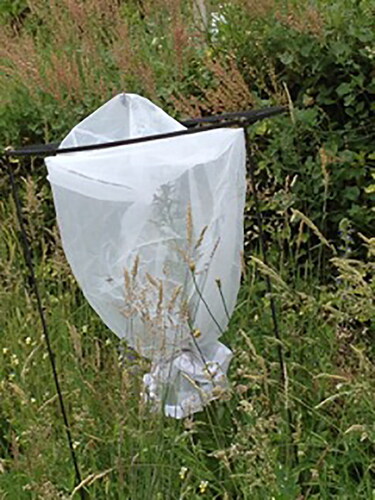
Figure 50. Structure of a floret and a floral head of E. cannabinum.

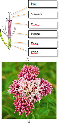
Figure 51. An E. cannabinum plant bagged with a net.

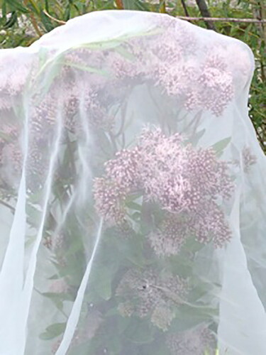
Figure 52. Extracted ion chromatograms of PAs identified in plant pollen of E. vulgare (A) and E. cannabinum (B). Peak numbers correspond to the PAs described in Table 51 (1: echimidine-N-oxide; 2: vulgarine-N-oxide; 3: acetylechimidine-N-oxide; 4: acetylvulgarine-N-oxide; 5: echivulgarine-N-oxide; 6: lycopsamine; 7: intermedine; 8-9: lycopsamine-N-oxide or intermedine-N-oxide).

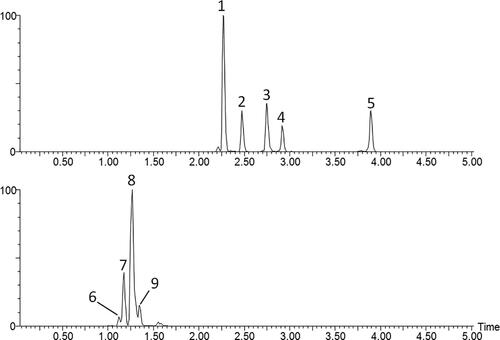
Table 52. Frequency of each plant genus as predominant pollen, secondary pollen, important minor pollen and minor pollen in the 134 pollen samples mixture analyzed.

Genus	Predominant pollen (>45%)	Secondary pollen (15–45%)	Important minor pollen (3–15%)	Minor pollen (<3%)
Eucalyptus spp.	13	21	21	21
Prunus spp.	8	4	4	4
Rubus spp.	8	11	8	8
Castanea spp.	15	34	23	8
Trifolium spp.	0	6	11	19
Cistus spp.	53	17	6	4
Echium spp.	21	17	11	4
Kiwi spp.	2	0	4	11
Leontondon spp.	0	2	17	11
Quercus spp.	0	6	11	15
Erica spp.	2	4	6	2
Thymus spp.	2	0	11	2
Genista spp.	0	6	6	2
Lavandula spp.	0	4	13	0
Cytisus spp.	11	23	11	2

Table 49. Retention and mass characteristics of known Echium-type and Eupatorium-type PAs (free bases/-N-oxides and isomers).

PA peak n°	Compound Name	RT (min)	Chemical formula	[M + H]^+ experimental	[M + H]^+ calculated	Error (mDa)
	Echium vulgare
1	Echimidine	2.28	C20H31NO7	398.2184	398.2179	0.5
	Echimidine-N-oxide
		2.27	C20H31NO8	414.2126	414.2128	−0.2
	Acetylechimidine	2.74	C22H33NO8	440.2282	440.2284	−0.2
3	Acetylechimidine-N-oxide	2.71	C22H33NO9	456.2234	456.2234	0.0
	Echivulgarine	3.81	C25H37NO8	480.2575	480.2575	0.0
5	Echivulgarine-N-oxide	3.83	C25H37NO9	496.3402	496.3405	−0.3
	Vulgarine	2.33	C20H31NO7	398.2174	398.2179	−0.5
2	Vulgarine-N-oxide	2.43	C20H31NO8	414.2133	414.2128	0.5
	Acetylvulgarine	2.88	C22H33NO9	440.2285	440.2284	0.1
4	Acetylvulgarine-N-oxide	2.87	C22H33NO9	456.2243	456.2234	0.9
	Eupatorium cannabinum
6	Lycopsamine	1.12	C15H25NO5	300.1807	300.1811	−0.4
7	Intermedine	1.16	C15H25NO5	300.1810	300.1811	−0.1
8	Lycopsamine-N-oxide or Intermedine-N-oxide*
		1.27	C15H25NO6	316.1756	316.1760	0.4
9	Lycopsamine-N-oxide or Intermedine-N-oxide*	1.35	C15H25NO6	316.1758	316.1760	0.2

* Distinction between the N-oxides of intermedine and lycopsamine not possible due to the lack of standards.

Figure 53. (a–d) Scheme of sample preparation for analysis in FTIR-ATR equipment.

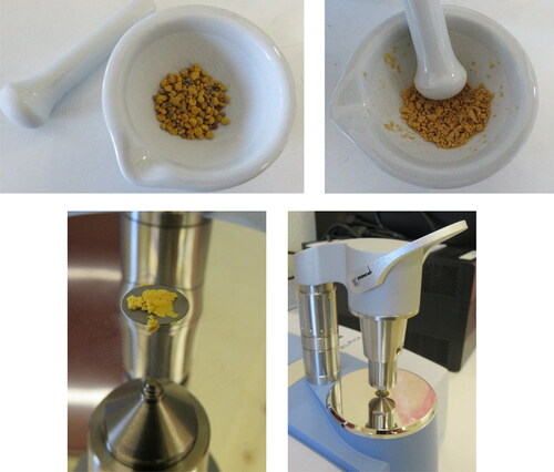
Figure 54. Average ATR spectrum of pollen samples.

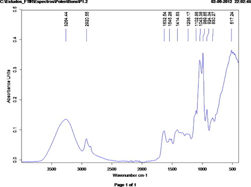
Table 53. Statistics of the 134 sample of bee pollen analyzed.

Parameter	Mean ± σ	Min − max	Coefficient of variation
Total phenolic compounds	23.9 ± 4.16	16.1–35.5	17.4
Total flavonoids	4.1 ± 0.96	2.2–5.9	23.2
EC50	3.5 ± 1.05	2.0–6.4	39.1
ABTS	244.9 ± 24.40	203.8–298.6	10.0

Table 54. Results for calibration and cross-validation.

Calibration
Parameter	Spectral range (cm^−1)	Pre-processing	Rk	r^2	RMSEE	RPD
Total phenolic compounds	2787 − 2459 + 2135 − 1809	2ndDer	8	92.6	1.16	3.7
Total flavonoids	2858 − 2509 + 2164 − 1470 + 777 − 430	VecNor	9	85.9	0.373	2.7
EC50	3055 − 2731 + 2087 − 1119 + 799 − 474	VecNor	10	89.7	0.351	3.1
ABTS	2557 − 1838 + 1479 − 399	1stDer	10	91.3	7.57	3.4
Cross-validation
Parameter	Spectral range(cm^−1)	Pre-processing	Bias	r^2	RMSECV	RPD
Total phenolic compounds	2787 − 2459 + 2135 − 1809	2ndDer	0.0044	79.3	1.88	2.2
Total flavonoids	2858 − 2509 + 2164 − 1470 + 777 − 430	VecNor	−0.0020	76.0	0.469	2.0
EC50	3055 − 2731 + 2087 − 1119 + 799 − 474	VecNor	0.0185	77.9	0.492	2.1
ABTS	2557 − 1838 + 1479 − 399	1stDer	0.2470	72.5	12.7	1.9

2ndDer – seconded derivative; VecNor – vector normalization; 1stDer – first derivative; r² – coefficient of determination; Rk – number of PLS components; RMSEE – root mean square error of calibration; RPD – residual prediction deviation; Bias – mean value of deviation, also called systematic error; RMSECV – root mean square error of cross-validation.

Table 55. Condition variations of the DPPH* assay on bee pollen according to different authors.

Number of report	Reference	Initial DPPH* concentration	Reaction time	Expression of activity	DPPH* volume/extract volume
1	Campos et al. (1997)	5.91 mg/250 ml in ethanol	10 min	EC50	2.5 ml-DPPH* solution + 1 to 10 µl extract
2	Kroyer and Hegedus (2001)	6 × 10^−5 M in methanol	60 min	% inhibition	2.7 ml-DPPH* solution + 0.3 ml extract
3	Nagai et al. (2002)	1 mM	NI	% activity	0.3 ml-DPPH* solution + 2.4 ml ethanol + 0.3 ml extract
4	Campos et al. (2003)	6 × 10^−5 M in methanol	10 min	EC50	2 ml-DPPH* solution + appropriate amount of extract
5	Almaraz-Abarca et al. (2004)	3.4 µg/ml in 50% etanol (v/v)	10 min	EC50	1600 to 1990 µl-DPPH* solution + 10 to 400 µl extract. Final volume: 2 ml
6	Nagai et al. (2005)	1 mM	NI	% activity	0.3 ml-DPPH* solution + 2.4 ml etanol + 0.3 ml extract
7	Silva et al. (2006)	6 × 10^−5 M in ethanol	30 min	EC50	2 ml-DPPH* solution + appropriate amount of extract
8	Leja et al. (2007)	0.1 mM in ethanol	30 min	% inhibition	0.083% pollen in the reaction mixture
9	Baltrušaitytė et al. (2007)	6.5 × 10^−5 M in methanol	16 min	% inhibition	2 ml-DPPH* solution + 50 µl extract
10	Carpes et al. (2008)	0.5 mM in ethanol	100 min	% inhibition, EC50	0.3 ml-DPPH* solution + 3 ml ethanol + 0.5 ml extract
11	Silva et al. (2009)	100 µM in ethanol	30 min	EC50	2 ml-DPPH* solution + appropriate amount of extract
12	LeBlanc et al. (2009)	51 mg/100 ml in methanol	60 min	% activity, EC50	242.5 µl DPPH* solution + 280 µl ethanol + 72 µl extract
13	Lee et al. (2009)	10 mM	10 min	% scavenging effect	1 ml-DPPH* solution + 4 ml extract
14	Mărghitas et al. (2009)	0.02 mg/ml	15 min	% inhibition	200 µl-DPPH* solution + 40 µl extract
15	Wang et al. (2010)	0.5 mM in ethanol	30 min	% activity	0.5 ml-DPPH* solution + 0.5 ml acetate buffer (100 mM, pH 5.5) + 0.5 ml extract
16	Menezes et al. (2010)	0.5 mM in ethanol	30 min	% activity	4 ml-DPPH* solution + 100 µl extract
17	Morais et al. (2011)	6 × 10^−5 M in methanol	60 min	%-DPPH* discoloration, EC50	2.7 ml-DPPH* solution + 300 µl extract
18	Negri et al. (2011)	20 µg/ml in methanol	20 min	% activity	3.9 ml-DPPH* solution + 0.1 ml extract
19	Graikou et al. (2011)	70 µM in methanol	Until a plateau was reached	% activity, EC50	1 ml-DPPH* solution + 50 µl extract
20	Feás et al. (2012)	6 × 10^−5 M in methanol	60 min	% absorbance, EC50	2.7 ml-DPPH* solution + 0.3 ml extract
21	Chantarudee et al. (2012)	0.15 mM in methanol	60 min	% activity, EC50	50 µl-DPPH* solution + 50 µl extract
22	Mejías and Montenegro (2012)	0.02 mg/mL in methanol	NI	µg ascorbic acid equivalents/g sample	1.5 ml-DPPH* solution + 750 µl extract
23	Melo et al. (2012a)	NI	NI	% activity	NI
24	Melo et al. (2012b)	NI	NI	% activity	NI
25	Melo et al. (2012c)	NI	30 min	% inhibition	NI
26	Melo et al. (2012d)	NI	30 min	% inhibition	NI
29	Arruda (2013)	6 × 10^−5 M in ethanol	30 min	EC50	1.5 ml-DPPH* solution + 2.0 ml etanol + 0.5 ml extract
	Arruda et al. (2013)	NI	NI	EC50	NI
27	Montenegro et al. (2013)	0.02 mg/ml	15 min	µg ascorbic acid equivalents/g pollen	1.5 ml-DPPH* solution + 0.75 ml extract
28	Cheng et al. (2013)	0.1 mM in methanol	30 min	% inhibition	4 ml-DPPH* solution + variable volumes of extract. Final volume: 10 ml
30	Ulusoy and Kolayli (2014)	0.1 mM in methanol	50 min	SC50	1.5 ml-DPPH* solution + 1.5 ml extract
31	Melo et al. (2013)	NI	30 min	IC50	NI
32	Barriada-Bernal et al. (2014)	40 µg/ml in ethanol	30 min	EC50	600 to 990 µl-DPPH* solution + 10 to 400 µl extract. Final volume: 1 m

NI = Not indicated.

Table 56. Advantages and disadvantages of some techniques and methods used for anti-microbial analysis.

Methods	Advantages	Disadvantages	References
Agar Diffusion	The technique works well with defined inhibitors; Flexibility in selection of disks for testing; Its simplicity of implementation and it is the least costly of all susceptibility methods; For testing of antifungal susceptibility its relative ease; Does not require for specialized equipment; Has intrinsic flexibility by being able to test the drugs the laboratory chooses; The provision of categorical results easily interpreted by all clinicians; The disk test has been standardized for testing not all fastidious or slow growing bacteria but, for some as streptococci, Haemophilus influenzae, and N. meningitides.	Less sensitive than micro-dilution techniques; Requires much quantity of sample for analysis; The antimicrobial effect may be inhibited or increased by extrinsic factors or contaminants as the type of agar and his concentration, salt concentration, incubation temperature, and molecular size of the antimicrobial component; There are substances in the culture medium that influence the test susceptibility as thymidine that antagonizes the activity of sulfonamides and trimetroprinas, leading to a false result of resistance to such agents; This technique also does not distinguish between bactericidal and bacteriostatic effects; The pH of the culture medium should be compatible with the microbial growth because the increase in acidity of the medium decreases the antibacterial activity. By another side, increases the activity of acidic substances such as penicillin; The minimum inhibitory concentration (MIC) cannot be determined; Is difficult to examine the susceptibility of fastidious and slow-growing bacteria; It is labor-intensive and time-consuming; Can represent an expensive approach if more than a few drugs are tested; The lack of mechanization or automation of the test.	Hewitt and Vincent (1989); Marsh and Goode (1994); Eloff (1998); Scorzoni et al. (2007); Rex et al. (2001); Ostrosky et al. (2008); Barry and Thornsberry (1991); Klancnik et al. (2010); Wilkins and Thiel (1973); Jiang (2011); Jorgensen and Ferraro (2009).
Macrodilution	-Generation of a quantitative result (i.e., the MIC); -Ease of performance; -Economy; -More rapid results, therefore their development could be highly desirable.	Requires large volumes of antibiotic; It is not recommend using for most routine procedures; Time consuming; It is tedious; Manual task of preparing the antibiotic solutions for each test; The possibility of errors in preparation of the antibiotic solutions; Relatively large amount of reagents and space; Generate large amounts of waste.	Jorgensen and Ferraro (2009); CLSI (2008); Wiegand et al. (2008); Ostrosky et al. (2008).
Micro-dilution in microtiter plate (96 wells)	The method is robust, is not expensive; Gives reproducible results and convenience of having pre-prepared panels; Is ca. 32 times more sensitive than other methods used in the literature; Requires a small/minimal quantity of reagents, samples and space that occurs due to the miniaturization of the test; Can be used for large numbers of samples; Can test the susceptibility of multiple antimicrobials at the same time; Enables a larger number of replicates, increasing the ability of confident results; Does not require high levels of skill; Leaves a permanent record; It decreases the intensive labor and time cost compared with agar-based method; The considerable savings in media usage; Also allow assistance in generating computerized reports if an automated panel reader is used; Works better with antibiotics because no precipitate forms; Compared with agar-based method, broth microdilution can decrease much labor and time; Is conveniently used for routine antimicrobial susceptibility testing in clinical laboratory; Is a suitable and fast screening method for MIC determination compared to other methods.	The lack of or poor growth of many anaerobic microorganisms; Testing some fastidious anaerobes gives inconsistent and unreliable results because of poor growth of strains due to excessive exposure to oxygen during the set-up procedure; Some inflexibility of drug selections available in standard commercial panels.	Eloff (1998); Ostrosky et al. (2008); Clinical and Laboratory Standards Institute (CLSI) (2009); Jiang (2011); Jorgensen and Ferraro (2009).

Table 57. Summary of some antimicrobial effects of bee pollen.

Pharmacological activity	Susceptible microorganisms	Methods of determinations	References
	E. coli, S. aureus, B. cereus and P. aeruginosa	Agar well diffusion	Abouda et al. (2011)
	Fungi: Aspergillus fumigatus, Aspergillus niger and Aspergillus flavus. Yeasts: Candida albicans (C. albicans), Candida glabrata, Candida krusei and Rhodotorula mucilaginosa. Bacteria: E. coli, S. aureus, Salmonella entérica (S. entérica), P. aeruginosa and Listeria monocytogenes (L. monocytogenes)	“	Kacániová et al. (2012)
	L. monocytogenes, S. entérica, E. coli, S. aureus and P. aeruginosa	“	Fatrcová-Šramková et al. (2013)
	Clostridium butyricum, Clostridium perfringens, Clostridium hystoliticum, Clostridium intestinale and Clostridium ramosum	“	Kacániová et al. (2014)
	Paenibacillus larvae, Bacillus subtilis (B. subtilis), B. cereus , E. coli and P. aeruginosa	“	Barbosa et al. (2006)
	S. aureus and Streptococcus pyogenes	“	Cabrera and Montenegro (2013)
	Enterobacteriaceae genera	“	Hleba et al. (2013)
	S. aureus and Staphylococcus epidermidis	“	Baltrušaityte et al. (2007)
	Viridans streptococci	“	Tichy and Novak (2000)
	Agrobacterium tumefaciens, P. syringae pv. tomato, X. axonopodis pv. Vesicatória, E. amylovora, P. corrugata, R. solanacearum, X. campestris pv. Campestris, A. vitis, C. michiganensis subsp. Michiganensis, E. carotovora pv. carotovora, P. savastanoi pv. savastanoi, P. syringae pv. Phaseolicola, P. syringae pv. syringae	Paper Disk diffusion	Basim et al. (2006)
	S. aureus, B. subtilis, P. aeruginosa, Klebsiella sp. and B. cereus	“	Carpes et al. (2007)
	S. aureus, B. Cereus, B. Subtillis, P. aeruginosa and K. Pneumoniae	“	Basuny et al. (2013)
	E. coli, S. aureus, B. subtilis, P. aeruginosa, K. pneumonia, Shigella flexneri, Salmonella typhi and Proteus mirabilis	“	Eswaran and Bhargava (2014)
	S. thyphimurium and E. coli.	“	Yerlikaya (2014)
	S. aureus [ATCC 29213], E. coli [ATCC 27853], Enterococcus faecalis [ATCC 29212], or P. aeruginosa [ATCC 25922]	Microdilution in Microtiter plate	Eloff (1998)
	S. aureus, S. epidermidis, E. coli, Enterobacter cloacae, Klebsiella pneumonia, P. aeruginosa, C. albicans, C. tropicalis and C. glabrata	“	Graikou et al. (2011)
	Salmonella typhi, S. aureus, B. cereus, E. coli, Zygosacharomyces mellis, Zygosacharomyces bailii, Zygosacharomyces rouxii and Candida magnolia	“	Morais et al. (2011)
	S. aureus, P. aeruginosa, E. coli and C. glabrata	“	Pascoal et al. (2014)

Figure 55. Inhibition zones around the disks.

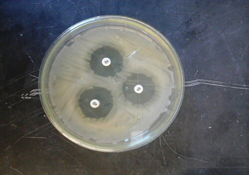
Figure 56. Inhibition zone around the well diffusion.

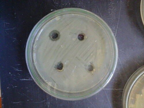
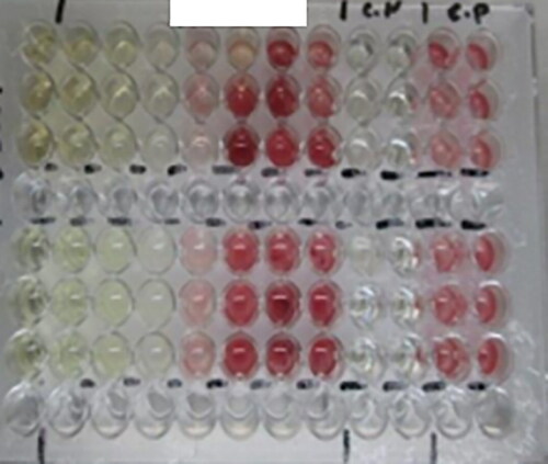
Figure 57. Microtiter plate (96 wells), showing the color change indicating the reduction of TTC by microorganisms.

Nôžková, J., Brindza, J., Ostrovský, R., Stehlíková, B., & Fatrcová-Šramková, K. (2010). Hodnotenie kvantitatívnych a kvalitatívnych znakov včelieho peľu a ich klasifikácia podľa navrhnutých deskriptorov: Evaluation of quantitative and qualitative traits of bee pollen and their classification according to proposed list of descriptors. In Potravinárstvo. Združenie HACCP Consulting 2007: Nitrianske Hrnčiarovce, Slovensko. 4, 204–216.

 Google Scholar

Sawyer, R. (1981). Pollen identification for beekeepers (p. 112). University College Cardiff Press.

 Google Scholar

Vorwohl, G. (1990). Progress, problems and future tasks of Melissopalynologie. Apidologie, 21(5), 383–389. (Article in German). https://doi.org/https://doi.org/10.1051/apido:19900501

 Web of Science ®Google Scholar

Campos, M. G., & Markham, K. R. (2007). Structure information from HPLC and on-line measured absorption spectra: Flavones, flavonols and phenolic acids. Imprensa da Universidade de Coimbra. https://doi.org/https://doi.org/10.14195/978-989-26-0480-0

 Google Scholar

Campos, M. G., Markham, K. R., Mitchell, K. A, & da Cunha, A. P. d. (1997). An approach to the characterization of bee pollens via their flavonoid/phenolic profiles. Phytochemical Analysis, 8(4), 181–185. https://doi.org/https://doi.org/10.1002/(SICI)1099-1565(199707)8:4 < 181::AID-PCA359 > 3.0.CO;2-A

 Web of Science ®Google Scholar

Serra-Bonvehí, J., Torrentó, S. M., & Lorente, C. E. (2001). Evaluation of polyphenolic and flavonoid compounds in honey bee – Collected pollen produced in Spain. Journal of Agricultural and Food Chemistry, 49(4), 1848–1853. https://doi.org/https://doi.org/10.1021/jf0012300

 PubMed Web of Science ®Google Scholar

Fanali, C., Dugo, L., & Rocco, A. (2013). Nano-liquid chromatography in nutraceutical analysis: determination of polyphenols in bee pollen. Journal of Chromatography. A, 1313, 270–274. https://doi.org/https://doi.org/10.1016/j.chroma.2013.06.055

 PubMed Web of Science ®Google Scholar

Di Paola-Naranjo, R. D., Sánchez, S. J., Paramás, A. M. G., & Rivas Gonzalo, J. C. (2004). Liquid chromatographic-mass spectrometric analysis of anthocyanin composition of dark blue bee pollen from Echium plantagineum. Journal of Chromatography. A, 1054(1-2), 205–210. https://doi.org/https://doi.org/10.1016/j.chroma.2004.05.023

 PubMed Web of Science ®Google Scholar

Ferreres, F., Pereira, D. M., Valentão, P., & Andrade, P. B. (2010). First report of non-coloured flavonoids in Echium plantagineum bee pollen: Differentiation of isomers by liquid chromatography/ion trap mass spectrometry. Rapid Communications in Mass Spectrometry, 24(6), 801–806. https://doi.org/https://doi.org/10.1002/rcm.4454

 PubMed Web of Science ®Google Scholar

Negri, G., Teixeira, E., Alves, M. L. T. F., Moreti, A. C. C. C., Otsuk, I. P., Borguini, R. G., & Salatino, A. (2011). Hydroxycinnamic acid amide derivatives, phenolic compounds and antioxidant activities of extracts of pollen samples from Southeast Brazil. Journal of Agricultural and Food Chemistry, 59(10), 5516–5522. https://doi.org/https://doi.org/10.1021/jf200602k

 PubMed Web of Science ®Google Scholar

Lv, H., Wang, X., He, Y., Wang, H., & Suo, Y. (2015). Identification and quantification of flavonoid aglycones in rape bee pollen from Qinghai-Tibetan Plateau by HPLC-DAD-APCI/MS. Journal of Food Composition and Analysis, 38, 49–54. https://doi.org/https://doi.org/10.1016/j.jfca.2014.10.011

 Web of Science ®Google Scholar

Herbert, E. W. J., & Shimanuki, H. (1978). Chemical composition and nutritive value of bee-collected and bee-stored pollen. Apidologie, 9(1), 33–40. https://doi.org/https://doi.org/10.1051/apido:19780103

 Web of Science ®Google Scholar

Serra-Bonvehí, J., & Escolá Jordá, R. (1997). Nutrient composition and microbiological quality of honey bee-collected pollen in Spain. Journal of Agricultural and Food Chemistry, 45(3), 725–732. https://doi.org/https://doi.org/10.1021/jf960265q

 Web of Science ®Google Scholar

Somerville, D. C. (2001). Nutritional value of bee collected pollens, a report for the Rural Industries Research and Development Corporation # 01/047 (pp. 57–58). NSW Agriculture Goulburn.

 Google Scholar

Villanueva, M. T. O., Díaz Marquina, A., Bravo Serrano, R., & Blazquez Abellán, G. (2002). The importance of bee-collected pollen in the diet: A study of its composition. International Journal of Food Sciences and Nutrition, 53(3), 217–224. https://doi.org/https://doi.org/10.1080/09637480220132832

 PubMed Web of Science ®Google Scholar

Andrada, A. C., & Telleria, M. C. (2005). Pollen collected by honey bees (Apis mellifera L.) from south of Caldén district (Argentina): Botanical origin and protein content. Grana, 44(2), 115–122. https://doi.org/https://doi.org/10.1080/00173130510010459

 Web of Science ®Google Scholar

Almeida-Muradian, L. B., Pamplona, L. C., Coimbra, S., & Barth, O. M. (2005). Chemical composition and botanical evaluation of dried bee pollen pellets. Journal of Food Composition and Analysis, 18(1), 105–111. https://doi.org/https://doi.org/10.1016/j.jfca.2003.10.008

 Web of Science ®Google Scholar

Szczêsna, T. (2006a). Long – Chain fatty acids composition of honey bee-collected pollen. Journal of Apicultural Science, 50, 65–78.

 Google Scholar

Szczêsna, T. (2006b). Protein content and amino acid composition of bee-collected pollen from selected botanical origins. Journal of Apicultural Science, 50, 81–90.

 Google Scholar

Forcone, A., Aloisi, P. V., Ruppel, S., & Munoz, M. (2011). Botanical composition and protein content of pollen collected by Apis mellifera L. in the north-west of Santa Cruz (Argentinean Patagonia). Grana, 50(1), 30–39. https://doi.org/https://doi.org/10.1080/00173134.2011.552191

 Web of Science ®Google Scholar

Martins, M. C. T., Morgano, M. A., Vincente, E., Baggio, S. R., & Rodriguez-Amaya, D. B. (2011). Physicochemical composition of bee pollen from eleven Brazilian states. Journal of Apicultural Science, 55(2), 107–116.

 Web of Science ®Google Scholar

Balkanska, R. G., Ignatova, M. M. (2012). Chemical composition of multifloral bee pollen from Bulgaria. In Proceedings of 6th Central European Congress on Food, CE Food 2012 (pp. 375–378).

 Google Scholar

Stanciu, O. G., Marghitas, L. A., & Dezmirean, D. (2012). Nutritional and biological values of bee pollen and beebread harvested from Romania. In Proceedings of International Conference of Agricultural Engineering CIGR-AGENG. http://journals.usamvcluj.ro/index.php/zootehnie/article/viewFile/9391/7820

 Google Scholar

Arruda, V. A. S., Freitas, A. S., B., O. M., Estevinho, L. M., & Almeida-Muradian, L. B. (2013). Propriedades biológicas do pólen apícola de coqueiro, coletado na Região Nordeste do Brasil. Magistra, 25, 1–6.

 Google Scholar

Liolios, V., Tananaki, C., Dimou, M., Kanelis, D., Goras, G., Karazafiris, E., Thrasyvoulou, A. (2014). Predict the chemical composition of pollen. In Proceedings of International Symposium on Bee Products, 3rd edition, September 28th – October 1st, p. 28.

 Google Scholar

Kozich, J. J., Westcott, S. L., Baxter, N. T., Highlander, S. K., & Schloss, P. D. (2013). Development of a dual-index sequencing strategy and curation pipeline for analyzing amplicon sequence data on the MiSeq Illumina sequencing platform. Applied and Environmental Microbiology, 79(17), 5112–5120. https://doi.org/https://doi.org/10.1128/AEM.01043-13

 PubMed Web of Science ®Google Scholar

Pantelić, M., Dabić, D., Matijašević, S., Davidović, S., Dojčinović, B., Milojković-Opsenica, D., Tešić, Ž., & Natić, M. (2014). Chemical characterization of fruit wine made from Oblačinska sour cherry. The Scientific World Journal, 2014, 454797–454799. https://doi.org/https://doi.org/10.1155/2014/454797

 Web of Science ®Google Scholar

Echigo, T., Takenaka, T., & Yatsunami, K. (1986). Comparative studies on chemical composition of honey, royal jelly and pollen loads. Bulletin of the Faculty of Agriculture Tamagawa University, 26, 1–8.

 Google Scholar

Melo, E. A., Filho, J. M., & Guerra, N. B. (2005) Characterization of antioxidant compounds in aqueous coriander extract (Coriandrum sativum L.). LWT—Food Science and Technology, 38, 15–19. https://doi.org/https://doi.org/10.1016/j.lwt.2004.03.011.

 Web of Science ®Google Scholar

Szczêsna, T. (2006c). Protein content and amino acids composition of bee-collected pollen originating from Poland, South Korea and China. Journal of Apicultural Science, 50, 91–99.

 Google Scholar

Hartmann, T., & Witte, L. (1995). Chemistry, biology and chemoecology of the pyrrolizidine alkaloids. In S. W. Pelletier (Ed.), Alkaloids: Chemical and biological perspectives (Vol. 9, pp. 155–233). Pergamon Press. https://doi.org/https://doi.org/10.1016/b978-0-08-042089-9.50011-5

 Google Scholar

Human, H., & Nicolson, S., W. (2006). Nutritional content of fresh, bee-collected and stored pollen of Aloe greatheadii var. davyana (Assphodelaceae). Phytochemistry, 67(14), 1486–1492. https://doi.org/https://doi.org/10.1016/j.phytochem.2006.05.023

 PubMed Web of Science ®Google Scholar

Nogueira, C., Iglesias, A., Feas, X., & Estevinho, L. M. (2012). Commercial bee pollen with different geographical origins: A comprehensive approach. International Journal of Molecular Sciences, 13(9), 11173–11187. https://doi.org/https://doi.org/10.3390/ijms130911173

 PubMed Web of Science ®Google Scholar

Kostić, A. Ž., Barać, M. B., Stanojević, S. P., Milojković-Opsenica, D. M., Tešić, Ž. L., Šikoparija, B., Radišić, P., Prentović, M., & Pešić, M. B. (2015). Physicochemical composition and techno-functional properties of bee pollen collected in Serbia. LWT – Food Science and Technology, 62(1), 301–309. https://doi.org/https://doi.org/10.1016/j.lwt.2015.01.0310023-6438

 Web of Science ®Google Scholar

Szczęsna, T., Rybak-Chmielewska, H., & Chmielewski, W. (2002). Sugar composition of pollen loads harvested at different periods of the beekeeping season. Journal of Apicultural Science, 46(2), 107–115.

 Google Scholar

Szczęsna, T. (2007). Study on the sugar composition of honey-bee-collected pollen. Journal of Apicultural Science, 51(1), 15–21.

 Google Scholar

Qian, W. L., Khan, Z., Watson, D. G., & Fearnley, J. (2008). Analysis of sugars in bee pollen and propolis by ligand exchange chromatography in combination with pulse amperometric detection and mass spectrometry. Journal of Food Composition and Analysis, 21(1), 78–83. https://doi.org/https://doi.org/10.1016/j.jfca.2007.07.001

 Web of Science ®Google Scholar

Bobis, O., Marghitas, L., Al, Dezmirean, D., Morar, O., Bonta, V., & Chirila, F. (2010). Quality parameters and nutritional value of different commercial bee products. Bulletin UASVM Animal Science and Biotechnologies, 67(1-2), 91–96.

 Google Scholar

Mărgăoan, R., Mărghitas, L., Al, Dezmirean, D. S., Bobis, O., & Mihai, C. M. (2012). Physical-Chemical composition of fresh bee pollen from Transylvania. Bulletin UASVM Animal Science and Biotechnologies, 69(1-2), 351–355.

 Google Scholar

Taha, E. A. (2015). Chemical composition and amounts of mineral elements in honey bee-collected pollen in relation to botanical origin. Journal of Apicultural Science, 59(1), 75–81. https://doi.org/https://doi.org/10.1515/JAS-2015-0008

 Web of Science ®Google Scholar

Oliveira, K. C. L. S., Moriya, M., Azedo, R. A. B., Almeida-Muradian, L. B., Teixeira, E. W., Alves, M. L. T. M. F., & Moreti, A. C. C. C. (2009). Relationship between botanical origin and antioxidants vitamins of bee-collected pollen. Química Nova, 32(5), 1099–1102. https://doi.org/https://doi.org/10.1590/S0100-40422009000500003

 Web of Science ®Google Scholar

Melo, I. L. P., Freitas, A. S., Barth, O. M., & Almeida-Muradian, L. B. (2009). Relação entre a composição nutricional e a origem floral de pólen apícola desidratado. [Correlation between nutritional composition and floral origin of dried bee pollen]. Revista Do Instituto Adolfo Lutz, 68, 346–353.

 Google Scholar

Melo, I. L. P., & Almeida-Muradian, L. B. (2010). Stability of antioxidants vitamins in bee pollen samples. Química Nova, 33(3), 514–518. https://doi.org/https://doi.org/10.1590/S0100-40422010000300004

 Web of Science ®Google Scholar

Kroyer, G., & Hegedus, N. (2001). Evaluation of bioactive properties of pollen extracts as functional dietary food supplement. Innovative Food Science & Emerging Technologies, 2(3), 171–174. https://doi.org/https://doi.org/10.1016/S1466-8564(01)00039-X

 Google Scholar

Nagai, T., Inoue, R., Inoue, H., & Suzuki, N. (2002). Scavenging capacities of pollen extracts from Cistus ladanifeus on autoxidation, superoxide radicals, hydroxyl radicals, and DPPH radicals. Nutrition Research, 22(4), 519–526. https://doi.org/https://doi.org/10.1016/S0271-5317(01)00400-6

 Web of Science ®Google Scholar

Campos, M. G., Webby, R. F., Markham, K. R., Mitchell, K. A., & da Cunha, A. P. (2003). Age-induced diminution of free radical scavenging capacity in bee pollens and the contribution of constituent flavonoids. Journal of Agricultural and Food Chemistry, 51(3), 742–745. https://doi.org/https://doi.org/10.1021/jf0206466

 PubMed Web of Science ®Google Scholar

Almaraz-Abarca, N., Campos, M. d. G., Ávila-Reyes, J. A., Naranjo-Jimenez, N., Herrera-Corral, J., & Gonzalez, V. L. S. (2004). Variability of antioxidant activity among honey bee-collected pollen of different botanical origin. Interciencia, 29(10), 574–578. doi: 0378-1844/04/10/574-05.

 Web of Science ®Google Scholar

Nagai, T., Nagashima, T., Suzuki, N., & Inoue, R. (2005). Antioxidant activity and angiotensin I-converting enzyme inhibition by enzymatic hydrolysates from bee bread. Zeitschrift fur Naturforschung. C, Journal of Biosciences, 60(1-2), 133–138. https://doi.org/https://doi.org/10.1515/znc-2005-1-224

 PubMed Web of Science ®Google Scholar

Silva, T. M. S., Camara, C. A., da Silva Lins, A. C., Maria Barbosa-Filho, J., da Silva, E. M. S., Freitas, B. M., & de Assis Ribeiro dos Santos, F. (2006). Chemical composition and free radical scavenging activity of pollen loads from stingless bee Melipona subnituda Ducke. Journal of Food Composition and Analysis, 19(6-7), 507–511. https://doi.org/https://doi.org/10.1016/j.jfca.2005.12.011

 Web of Science ®Google Scholar

Leja, M., Mareczek, A., Wyżgolik, G., Klepacz-Baniak, J., & Czekońska, K. (2007). Antioxidative properties of bee pollen in selected plant species. Food Chemistry, 100(1), 237–240. https://doi.org/https://doi.org/10.1016/j.foodchem.2005.09.047

 Web of Science ®Google Scholar

Baltrušaitytė, V., Venskutonis, P. R., & Čeksterytė, V. (2007b). Radical scavenging activity of different floral origin honey and beebread phenolic extracts. Food Chemistry, 101(2), 502–514. https://doi.org/https://doi.org/10.1016/j.foodchem.2006.02.007

 Web of Science ®Google Scholar

Carpes, S. T., Prado, A. P., Moreno, I. A. M., Mourão, G. B., DE Alencar, S. M., & Masson, M. L. (2008). Avaliação do potencial antioxidante do pólen apícola producido na região sul do Brasil. Química Nova, 31(7), 1660–1664. https://doi.org/https://doi.org/10.1590/S0100-40422008000700011

 Web of Science ®Google Scholar

Silva, T. M. S., Camara, C. A., Lins, A. C. S., Agra, M. F., Silva, E. M. S., Reis, I. T., & Freitas, B. M. (2009). Chemical composition, botanical evaluation and screening of radical scavenging activity of collected pollen by the stingless bees Melipona rufiventris (Uruçu-amarela)). Anais da Academia Brasileira de Ciencias, 81(2), 173–178. https://doi.org/https://doi.org/10.1590/s0001-37652009000200003

 PubMed Web of Science ®Google Scholar

LeBlanc, B. W., Davis, O. K., Boue, S., DeLucca, A., & Deeby, T. (2009). Antioxidant activity of Sonoran Desert bee pollen. Food Chemistry, 115(4), 1299–1305. https://doi.org/https://doi.org/10.1016/j.foodchem.2009.01.055

 Web of Science ®Google Scholar

Lee, K.-H., Kim, A.-J., & Choi, E.-M. (2009). Antioxidant and anti-inflammatory activity of pine pollen extract in vitro. Phytotherapy Research, 23(1), 41–48. https://doi.org/https://doi.org/10.1002/ptr.2525

 PubMed Web of Science ®Google Scholar

Wang, S., Xie, B., Yin, L., Duan, L., Li, Z., Eneji, A. E., Tsuji, W., & Tsunekawa, A. (2010). Increased UV-B radiation affects the viability, reactive oxygen species accumulation and antioxidant enzyme activities in maize (Zea mays L.) pollen. Photochemistry and Photobiology, 86(1), 110–116. https://doi.org/https://doi.org/10.1111/j.1751-1097.2009.00635.x

 PubMed Web of Science ®Google Scholar

Menezes, J. D. S., Maciel, L. F., Miranda, M. S., & Druzian, J. I. (2010). Compostos bioactivos e potencial antioxidante de pólen apícola producido por abelhas africanizadas (Apis mellifera L.). Revista do Instituto Adolfo Lutz, 69(2), 233–242.

 Google Scholar

Morais, M., Moreira, L., Feás, X., & Estevinho, L. M. (2011). Honeybee-collected pollen from five Portuguese Natural Parks: Palynological origin, phenolic content, antioxidant properties and antimicrobial activity. Food and Chemical Toxicology, 49(5), 1096–1101. https://doi.org/https://doi.org/10.1016/j.fct.2011.01.020

 PubMed Web of Science ®Google Scholar

Graikou, K., Kapeta, S., Aligiannis, N., Sotiroudis, G., Chondrogianni, N., Gonos, E., & Chinou, I. (2011). Chemical analysis of Greek pollen – Antioxidant, antimicrobial and proteasome activation properties. Chemistry Central Journal, 5(1), 33–39. https://doi.org/https://doi.org/10.1186/1752-153X-5-33

 PubMed Web of Science ®Google Scholar

Feás, X., Vázquez-Tato, M. P., Estevinho, L., Seijas, J. A., & Iglesias, A. (2012). Organic bee pollen: Botanical origin, nutritional value, bioactive compounds, antioxidant activity and microbiological quality. Molecules, 17(7), 8359–8377. https://doi.org/http://dx.doi.org/10.3390/molecules17078359

 PubMed Web of Science ®Google Scholar

Chantarudee, A., Phuwapraisirian, P., Kimura, K., Okuyama, M., Mori, H., Kimura, A., & Chanchao, C. (2012). Chemical constituents and free radical scavenging activity of corn pollen collected from Apis mellifera hives compared to floral corn pollen at Nam, Thailand. BMC Complementary & Alternative Medicine, 12, 45.

 PubMed Web of Science ®Google Scholar

Mejías, E., & Montenegro, G. (2012). The antioxidant activity of Chilean honey and bee pollen produced in the Llaima volcano’s zonez. Journal of Food Quality, 35(5), 315–322. https://doi.org/https://doi.org/10.1111/j.1745-4557.2012.00460.x

 Web of Science ®Google Scholar

Melo, A. A. M., Meira, D. F. S., Chan, J., Sattler, J. A. G., & Almeida-Muradian, L. B. (2012a). Comparação entre métodos de extração de compostos antioxidantes do pólen apícola desidratado. In: 11º Encontro de Química de Alimentos, Bragança. 11º Encontro de Química de Alimentos – Qualidade dos alimentos: novos desafios/Resumos, p. 65–65.

 Google Scholar

Melo, A. A. M., Meira, D. F. S., Sattler, J. A. G., & Almeida-Muradian, L. B. (2012b). Atividade antioxidante do pólen apícola desidratado avaliada por diferentes métodos de extração. Mensagem Doce (Associação Paulista de Apicultores, Criadores de Abelhas Melificas Européias), São Paulo, p. 59, 22 maio.

 Google Scholar

Melo, A. A. M., Meira, D. F. S., Sattler, J. A. G., & Almeida-Muradian, L. B. (2012c). Antioxidant activity of bee pollen produced in two Brazilian states [Paper presentation]. 5th European Conference of Apidology, Halle an Der Saale. EurBee 5 – 5th European Conference of Apidology (p. 223).

 Google Scholar

Melo, A. A. M., Meira, D. F. S., Sattler, J. A. G., Almeida-Muradian, L. B. (2012d). Antioxidant activity of dehydrated bee pollen produced in Rio Grande do Sul state, Brazil. In II International Symposium on Bee Products/Annual Meeting of IHC, Bragança/Book of Abstracts (p. 75).

 Google Scholar

Arruda, V. A. S. (2013). Dried bee pollen: Physicochemical, microbiological quality, phenolic and flavonoid compounds, antioxidant activity and botanical origin [PhD thesis]. Pharmaceutical Science School, University of São Paulo.

 Google Scholar

Montenegro, G., Pizarro, R., Mejías, E., & Rodríguez, S. (2013). Evaluación biológica de polen apícola de plantas de Chile. Revista Internacional de Botánica Experimental, 82, 7–14.

 Google Scholar

Ulusoy, E., & Kolayli, S. (2014). Phenolic composition and antioxidant properties of anzer bee pollen. Journal of Food Biochemistry, 38(1), 73–82. https://doi.org/http://dx.doi.org/10.1111/jfbc.12027 https://doi.org/https://doi.org/10.1111/jfbc.12027

 Web of Science ®Google Scholar

Melo, A. A. M., Nagai, M. K., Chan, J., & Almeida-Muradian, L. B. (2013). Chemical composition, total phenolic compounds and antioxidant activity of dehydrated bee pollen produced in four Brazilian states. In XXXXIII International Apicultural Congress. Apimondia – Scientific Program/Posters.

 Google Scholar

Barriada-Bernal, L. G., Almaraz-Abarca, N., Delgado-Alvarado, E. A., Gallardo-Velázquez, T., Ávila-Reyes, J. A., Torres-Morán, M. I., González-Elizondo, M. d. S., & Herrera-Arrieta, Y. (2014). Flavonoid composition and antioxidant capacity of the edible flowers of Agave durangensis (Agavaceae). Cyta – Journal of Food, 12(2), 105–114. https://doi.org/https://doi.org/10.1080/19476337.2013.801037

 Web of Science ®Google Scholar

Hewitt, W., & Vincent, S. (1989). Theory and application of microbiological assay. Academic Press.

 Google Scholar

Marsh, J., & Goode, J. A. (Eds.) (1994). Antimicrobial Peptides ICiba Foundation Symposium 186]. John Wiley & Sons.

 Google Scholar

Eloff, J. N. (1998). A sensitive and quick microplate method to determine the minimal inhibitory concentration of plant extracts for bacteria. Planta Medica, 64(8), 711–713. https://doi.org/https://doi.org/10.1055/s-2006-957563

 PubMed Web of Science ®Google Scholar

Scorzoni, L., Benaducci, T., Almeida, A. M. F., Silva, D. H. S., Bolzani, V. S., & Gianinni, M. J. (2007). The use of standard methodology for determination of antifungal activity of natural products against medical yeasts Candida sp. and Cryptococcus sp. Brazilian Journal of Microbiology, 38, 391–397. https://doi.org/https://doi.org/10.1590/S1517-83822007000300001.

 Web of Science ®Google Scholar

Rex, J. H., Pfaller, M. A., Walsh, T. J., Chaturvedi, V., Espinel-Ingroff, A., Ghannoum, M. A., Gosey, L. L., Odds, F. C., Rinaldi, M. G., Sheehan, D. J., & Warnock, D. W. (2001). Antifungal susceptibility testing: Practical aspects and current challenges. Clinical Microbiology Reviews, 14(4), 643–658. https://doi.org/https://doi.org/10.1128/CMR.14.4.643-658.2001

 PubMed Web of Science ®Google Scholar

Ostrosky, E. A., Mizumoto, M. K., Lima, M. E. L., Kaneko, T. M., Nishikawa, S. O., & Freitas, B. R. (2008). Métodos para avaliação da actividade antimicrobiana e determinação da concentração mínima inibitória (CMI) de plantas medicinais. Revista Brasileira de Farmacognosia, 18(2), 301–307. https://doi.org/https://doi.org/10.1590/S0102-695X2008000200026

 Google Scholar

Barry, A. L., & Thornsberry, C. (1991). Susceptibility tests: Diffusion test procedures. In A. Balows, W. J. Hauser, K. L. Hermann, H. D. Isenberg, & H. J. Shamody (Eds.), Manual of clinical microbiology (Vol. 5, pp. 1117–1125). American Society for Microbiology.

 Google Scholar

Klancnik, A., Piskernik, S., Jersek, B., & Mozina, S. S. (2010). Evaluation of diffusion and dilution methods to determine the antibacterial activity of plant extracts. Journal of Microbiological Methods, 81(2), 121–126. https://doi.org/https://doi.org/10.1016/j.mimet.2010.02.004

 PubMed Web of Science ®Google Scholar

Wilkins, T. D., & Thiel, T. (1973). Modified broth-disk method for testing the antibiotic susceptibility of anaerobic bacteria. Antimicrobial Agents and Chemotherapy, 3(3), 350–356. https://doi.org/https://doi.org/10.1128/AAC.3.3.350

 PubMed Web of Science ®Google Scholar

Jiang, L. (2011). Comparison of disk diffusion, agar dilution, and broth microdilution for antimicrobial susceptibility testing of five chitosans [Thesis in Master of Science]. Faculty of the Louisiana State University and Agricultural and Mechanical College, Department of Food Science.

 Google Scholar

Jorgensen, J. H., & Ferraro, M. J. (2009). Antimicrobial susceptibility testing: A review of general principles and contemporary practices. Clinical Infectious Diseases, 49(11), 1749–1755. https://doi.org/https://doi.org/10.1086/647952

 PubMed Web of Science ®Google Scholar

Wiegand, I., Hilpert, K., & Hancock, R. E. W. (2008). Agar and broth dilution methods to determine the minimal inhibitory concentration (MIC) of antimicrobial substances. Nature Protocols, 3(2), 163–175. https://doi.org/https://doi.org/10.1038/nprot.2007.521

 PubMed Web of Science ®Google Scholar

Clinical and Laboratory Standards Institute (CLSI). (2009). Performance standards for antimicrobial disk susceptibility tests; approved standard-tenth edition M02-A10. National Committee for Clinical Laboratory Standards, 29. 76 pp

 Google Scholar

Abouda, Z., Zerdani, I., Kalalou, I., Faid, M., & Ahami, M. T. (2011). The antibacterial activity of Moroccan bee bread and bee-pollen (fresh and dried) against pathogenic bacteria. Research Journal of Microbiology, 6(4), 376. https://doi.org/http://dx.doi.org/10.3923/jm.2011.376.384

 Google Scholar

Kacániová, M., Vuković, N., Chlebo, R., Haščík, P., Rovná, K., Cubon, J., Džugan, M., & Pasternakiewicz, A. (2012). The antimicrobial activity of honey, bee pollen loads and beeswax from Slovakia. Archives of Biological Sciences, 64(3), 927–934. https://doi.org/https://doi.org/10.2298/ABS1203927K

 Web of Science ®Google Scholar

Fatrcová-Šramková, K., Nôžková, J., Kačániová, M., Máriássyová, M., Rovná, K., & Stričík, M. (2013). Antioxidant and antimicrobial properties of monofloral bee pollen. Journal of Environmental Science and Health. Part. B, Pesticides, Food Contaminants, and Agricultural Wastes, 48(2), 133–138. https://doi.org/https://doi.org/10.1080/03601234.2013.727664

 PubMed Web of Science ®Google Scholar

Barbosa, S. I. T. R., Silvestre, A. J. D., Simões, M. M. Q., & Estevinho, M. L. (2006). Composition and antibacterial activity of the lipophilic fraction of honey bee pollen from native species of Montesinho Natural Park. International Journal of Agricultural Research, 1(5), 471–749.

 Google Scholar

Cabrera, C., & Montenegro, G. (2013). Pathogen control using a natural Chilean bee pollen extract of known botanical origin. Ciencia e Investigación Agraria, 40(1), 223–230. https://doi.org/https://doi.org/10.4067/S0718-16202013000100020

 Web of Science ®Google Scholar

Hleba, L., Pochop, J., Felšöciová, S., Petrová, J., Čuboň, J., Pavelková, A., & Kačániová, M. (2013). Antimicrobial effect of bee collected pollen extract to Enterobacteriaceae Genera after application of bee collected pollen in their feeding. Animal Science and Biotechnologies, 46(2), 108–113.

 Google Scholar

Tichy, J., & Novak, J. (2000). Detection of antimicrobials in bee products with activity against viridans streptococci. Journal of Alternative and Complementary Medicine, 6(5), 383–389. https://doi.org/https://doi.org/10.1089/acm.2000.6.383

 PubMed Web of Science ®Google Scholar

Basim, E., Basim, H., & Ozcan, M. (2006). Antibacterial activities of Turkish pollen and propolis extracts against plant bacterial pathogens. Journal of Food Engineering, 77(4), 992–996. https://doi.org/https://doi.org/10.1016/j.jfoodeng.2005.08.027

 Web of Science ®Google Scholar

Carpes, S. T., Begnini, R., DE Alencar, S. M., & Masson, M. L. (2007). Study of preparations of bee pollen extracts, antioxidant and antibacterial activity. Ciência e Agrotecnologia, 31(6), 1818–1825. https://doi.org/https://doi.org/10.1590/S1413-70542007000600032

 Web of Science ®Google Scholar

Basuny, A. M., Arafat, S. M., & Soliman, H. M. (2013). Chemical analysis of olive and palm pollen: Antioxidant and antimicrobial activation properties. Herald Journal of Agriculture and Food Science Research, 2(3), 091–097.

 Google Scholar

Eswaran, V. U., & Bhargava, H. R. (2014). Chemical analysis and anti-microbial activity of Karnataka bee bread of Apis species. World Applied Sciences Journal, 32(3), 379–385. https://doi.org/https://doi.org/10.5829/idosi.wasj.2014.32.03.1006

 Google Scholar

Yerlikaya, O. (2014). Effect of bee pollen supplement on antimicrobial, chemical, rheological, sensorial properties and probiotic viability of fermented milk beverages. Mljekarstvo, 64(4), 268–279. https://doi.org/https://doi.org/10.15567/mljekarstvo.2014.0406

 Web of Science ®Google Scholar

Pascoal, A., Rodrigues, S., Teixeira, A., Feás, X., & Estevinho, L. M. (2014). Biological activities of commercial bee pollens: Antimicrobial, antimutagenic, antioxidant and anti-inflammatory. Food and Chemical Toxicology, 63, 233–239. https://doi.org/https://doi.org/10.1016/j.fct.2013.11.010

 PubMed Web of Science ®Google Scholar