Experimental seabed disturbance effects on Chatham Rise deep-sea meiofaunal communities, Southwest Pacific

Figures & data

Figure 1. Map of (A) Aotearoa/New Zealand (inset) showing location of Chatham Rise, study area (black filled rectangle), Mid Chatham Rise Benthic Protection Area (BPA) and Chatham Rock Phosphate’s Mineral License and Mineral Permit areas (numbered), and (B) study area showing location of reference site (black X) and Butterknife feature (black rectangle), with multibeam echosounder backscatter background showing areas of high and low reflectivity (white and dark grey shading, respectively).

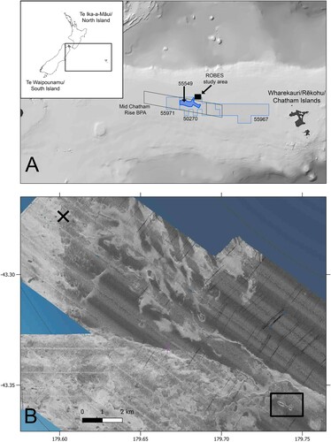
Figure 2. Butterknife feature showing location of directly disturbed sites (DI; grey filled circles), undisturbed or indirectly disturbed sites (UI; black diamonds), trajectory of Sediment Cloud Inducing Plow (SCIP) when in contact on the seabed (light blue) and location of the three landers (white crosses; L1-L3). Multibeam echosounder backscatter background shows areas of high and low reflectivity (white and dark grey shading, respectively).

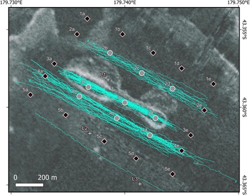
Figure 3. The Sediment Cloud Induction Plough (SCIP) used during the Butterknife disturbance experiment, showing (a) tickler chain, (b) tynes, and (c) harrow mat.

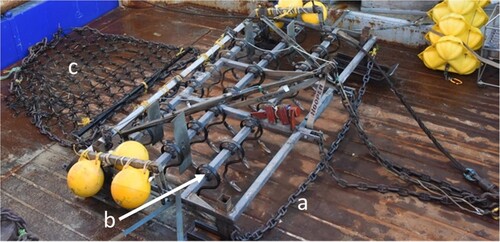
Table 1. Details of study sites on the Chatham Rise Butterknife feature during the ROBES voyages TAN1903 (Pre- and Post-disturbance) and TAN2005 (One year post-disturbance). DI = directly and indirectly disturbed; UI = undisturbed or indirectly disturbed; x = collected sample; ns = no sample.

Site	Longitude	Latitude	Water Depth (m)	Treatment	Pre-disturbance	Post-disturbance	One year post- disturbance
1a	179.7367	−43.3543	459	UI	x	x	x
1b	179.7398	−43.3553	461	UI	ns	ns	x
1c	179.7425	−43.3565	458	UI	x	x	x
1d	179.7450	−43.3575	458	UI	ns	ns	x
1e	179.7478	−43.3585	458	UI	x	x	x
2a	179.7358	−43.3553	459	UI	x	x	x
2b	179.7387	−43.3565	454	DI	ns	ns	x
2c	179.7415	−43.3578	453	DI	x	x	x
2d	179.7442	−43.3588	461	DI	ns	ns	x
2e	179.7470	−43.3602	460	UI	x	x	x
3a	179.7338	−43.3572	457	UI	ns	ns	x
3b	179.7368	−43.3587	460	DI	x	x	x
3c	179.7400	−43.3597	457	DI	x	x	x
3d	179.7427	−43.3607	467	DI	x	x	x
3e	179.7458	−43.3618	460	UI	ns	ns	x
4a	179.7330	−43.3580	458	UI	x	x	x
4b	179.7360	−43.3593	458	DI	ns	ns	x
4c	179.7393	−43.3607	457	DI	x	x	x
4d	179.7422	−43.3618	458	DI	ns	ns	x
4e	179.7450	−43.3628	456	UI	x	x	x
5a	179.7317	−43.3592	461	UI	ns	ns	x
5b	179.7348	−43.3605	455	UI	ns	x	x
5c	179.7382	−43.3622	458	UI	x	x	x
5d	179.7410	−43.3633	459	UI	x	x	x
5e	179.7442	−43.3643	458	UI	ns	ns	ns
REF	179.6022	−43.2737	455	Reference	x	ns	x

Figure 4. Turbidity measurements from three benthic landers positioned around the Butterknife. Benthic landers 1, 2 and 3 are labelled L1, L2 and L3, respectively. Lander 1 was positioned closest to the Butterknife and Lander 3 was furthest (see Figure 2). Red labels indicate the time at which sampling and disturbance events took place. FTU = Formazin Turbidity Unit (Nodder et al. in prep; see also Clark et al. 2019).

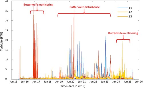
Figure 5. Sediment characteristics (C:N ratio, chlorophyll a (Chl a), total organic matter (TOM), mud content (%silt/clay) and water content (%H₂O)) at directly and indirectly disturbed (DI; grey bars), undisturbed or indirectly disturbed (UI; black bars) and reference sites (white bars) prior to disturbance, immediately post-disturbance, and one year post-disturbance (mean and standard deviation). Data for the 0–1 cm layer are shown on the left-hand side graphs and corresponding data for the 1–5 cm layer on the right-hand side graphs. White bars with dotted outline show values that were measured pre-disturbance at the reference site but shown next to post-disturbance bars for ease of comparison.

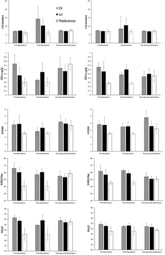
Table 2. PERMANOVA results showing significance testing for the effect of factors Time (Pre-disturbance, post-disturbance, and one year post-disturbance) and Disturbance (directly and indirectly disturbed (DI) versus undisturbed or indirectly disturbed (UI)) and their interaction on multivariate sediment parameters. Separate analyses were conducted for the 0–1 and 1–5 cm sediment layers as well as the two layers combined (0-5 cm).

Source	df	Sediment characteristics
		MS	Pseudo-F	P
0-1 cm
Time	2	63.076	6.009	0.001
Disturbance	1	3.7165	0.35405	0.910
Time x Disturbance	2	22.324	2.1267	0.043
Residuals	40
1-5 cm
Time	2	59.474	5.7434	0.001
Disturbance	1	10.513	1.0153	0.381
Time x Disturbance	2	6.9096	0.66727	0.778
Residuals	38
0-5 cm
Time	2	46.878	4.2085	0.001
Disturbance	1	10.489	0.94167	0.453
Time x Disturbance	2	13.854	1.2437	0.255
Residuals	40

Table 3. Results of SIMPER analyses showing the environmental factors responsible for differences among sampling times, i.e. pre- versus post-disturbance, pre – versus one year post-disturbance and post – versus one year post-disturbance, for the 0–1 and 1–5 cm sediment layers. % Cum. Contrib. = cumulative percentage contribution to dissimilarity in sediment characteristics. C:N = molar carbon to nitrogen ratio in sediment organic matter (i.e. molar POC:PN); TOM = %total organic matter; PN = %sediment particulate nitrogen; POC = %sediment particulate organic carbon; Silt/clay = %silt/clay; Chl a = sediment chlorophyll a in µg/g dry sediment; Phaeo = sediment phaeopigments in µg/g dry sediment.

	Pre-disturbance	Post-disturbance	Cum. Contrib. %		Pre-disturbance	One year post-disturbance	Cum. Contrib. %		Post-disturbance	One year post-disturbance	Cum. Contrib. %
0-1 cm
C:N	7.2	11.7	17	Silt/clay	62	54	13	C:N	11.7	7.2	18
TOM	3.8	3.1	29	TOM	3.8	4.1	24	POC	0.69	0.57	28
PN	0.08	0.06	40	PN	0.08	0.07	35	PN	0.06	0.07	38
POC	0.64	0.69	49	Mean grain size	62	71	44	TOM	3.2	4.1	47
1-5 cm
–				Silt/clay	59	52	12	C:N	9.1	7.5	16
–				Chl a	0.61	0.47	23	Phaeo	4.5	3.7	27
–				Mean grain size	65	74	33	POC	0.61	0.52	47
–				TOM	3.8	4.2	43	Silt/clay	62	52	47

Figure 6. Meiofaunal community parameters (abundance, richness, Shannon diversity H’10 and Pielou’s eveness J’) at directly and indirectly disturbed (DI; grey bars), undisturbed or indirectly disturbed (UI; black bars) and reference sites (white bars) prior to disturbance, immediately post-disturbance, and one year post-disturbance (mean and standard deviation). Data for the 0–1 cm layer are shown on the left-hand side graphs and corresponding data for the 1–5 cm layer on the right-hand side graphs. White bars with dotted outline show values that were measured pre-disturbance at the reference site but shown next to post-disturbance bars for ease of comparison.

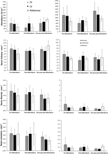
Table 4. Mean abundance (ind. 10 cm^-2) of meiofauna taxa at the Reference and Butterknife sites in surface (0-1 cm) and subsurface sediment layers (1-5 cm).

	Reference site		Butterknife sites
	0-1 cm	1-5 cm	0-1 cm	1-5 cm
Nematodes	505.68	803.68	458.39	1082.48
Copepods	36.34	8.07	41.93	7.40
Nauplii	27.47	5.80	36.45	5.08
Gastrotrichs	1.08	0.50	1.16	0.57
Polychaetes	8.00	7.57	33.05	6.80
Mites	0.22	–	0.82	0.29
Amphipods	0.22	0.25	0.87	0.14
Isopods	0.65	–	0.76	–
Tanaids	0.87	–	0.67	0.09
Ostracods	1.30	1.01	1.11	0.20
Kinorhynchs	4.11	0.50	6.17	1.60
Flatworms	–	–	0.23	0.03
Sipunculids	–	–	0.03	0.06
Tardigrades	–	–	0.15	–
Cnidarians	–	–	0.03	0.17
Gastropods	0.22	–	0.03	–
Aplacophorans	0.43	–	0.15	0.06
Nemerteans	-	0.25	0.03	0.11
Bivalves	0.22	–	–	–
Priapulids	-	–	–	0.09
Scaphopods	0.22	–	–	–
Ophiuroids	0.22	–	0.06	–

Table 5. Summary of meiofaunal univariate community parameters at the disturbed, undisturbed and reference sites sampled pre-, post-, and one year post-disturbance (means, and standard deviations in brackets). Data are shown for the 0–1 cm, 1–5 cm and combined 0–5 cm sediment layers. N = abundance 10 cm^-2; S = taxon richness; H′10 = Shannon diversity; J′ = taxon evenness.

	Sediment layer	Directly and indirectly disturbed (DI)			Undisturbed or indirectly disturbed (UI)			Reference
		Pre N = 5	Post N = 5	One year post N = 9	Pre N = 9	Post N = 10	One year post N = 15	Pre N = 3	One year post N = 3
N (10 cm^-2)	0-1 cm	342 (148)	336 (227)	558 (273)	720 (333)	484 (463)	733 (312)	320 (249)	894 (131)
	1-5 cm	884 (482)	547 (331)	1470 (637)	1298 (640)	781 (293)	1247 (528)	729 (275)	926 (192)
	0-5 cm	1226 (558)	883 (541)	2029 (820)	2018 (844)	1265 (612)	1980 (779)	1049 (499)	1820 (132)
S (core^−1)	0-1 cm	7.2 (1.3)	6.8 (0.8)	7.8 (0.8)	8.0 (1.6)	7.2 (1.0)	7.1 (1.4)	6.0 (2.0)	9.0 (1.7)
	1-5 cm	5.8 (1.5)	4.0 (0.7)	4.8 (1.2)	5.3 (1.6)	4.7 (1.6)	4.1 (1.4)	4.3 (0.6)	4.7 (2.9)
	0-5 cm	8.2 (1.6)	7.0 (0.7)	8.3 (0.7)	8.6 (1.8)	8.0 (1.2)	7.5 (1.4)	6.3 (1.5)	9.3 (2.1)
H′10	0-1 cm	0.42 (0.16)	0.29 (0.11)	0.33 (0.09)	0.34 (0.13)	0.36 (0.13)	0.24 (0.09)	0.30 (0.14)	0.24 (0.09)
	1-5 cm	0.13 (0.14)	0.06 (0.03)	0.04 (0.02)	0.07 (0.03)	0.08 (0.06)	0.03 (0.02)	0.05 (0.04)	0.08 (0.06)
	0-5 cm	0.24 (0.14)	0.17 (0.09)	0.16 (0.07)	0.18 (0.04)	0.21 (0.09)	0.12 (0.04)	0.14 (0.08)	0.17 (0.06)
J′	0-1 cm	0.50 (0.16)	0.35 (0.13)	0.37 (0.10)	0.38 (0.12)	0.42 (0.16)	0.29 (0.12)	0.42 (0.29)	0.26 (0.09)
	1-5 cm	0.17 (0.18)	0.08 (0.04)	0.06 (0.03)	0.09 (0.03)	0.11 (0.06)	0.05 (0.03)	0.08 (0.05)	0.13 (0.05)
	0-5 cm	0.26 (0.14)	0.20 (0.10)	0.17 (0.07)	0.19 (0.03)	0.23 (0.10)	0.14 (0.04)	0.18 (0.12)	0.18 (0.05)

Table 6. PERMANOVA results showing significance testing for the effect of factors Time (Pre-disturbance, post-disturbance, and one year post-disturbance) and Disturbance (directly and indirectly disturbed (DI) versus undisturbed or indirectly disturbed (UI)) and their interaction on meiofaunal community parameters. Separate analyses were conducted for the 0–1 and 1–5 cm sediment layers as well as the two layers combined (0-5 cm).

Source	df	Abundance (N)			Richness (S)			Shannon diversity (H’10)			Evenness (J’)			Community structure
		MS	Pseudo-F	P	MS	Pseudo-F	P	MS	Pseudo-F	P	MS	Pseudo-F	P	MS	Pseudo-F	P
0-1 cm
Time	2	103230	2.1937	0.115	0.99243	0.85141	0.43	0.040037	3.0948	0.064	0.048087	2.8579	0.068	1664.9	4.4553	0.003
Disturbance	1	271800	5.7759	0.02	0.88437	0.7587	0.385	0.016127	1.2466	0.278	0.022283	1.3244	0.255	763.03	2.0418	0.08
Time x Disturbance	2	24056	0.51121	0.595	3.9508	3.3894	0.055	0.028767	2.2236	0.126	0.033917	2.0158	0.148	602.46	1.6121	0.121
Residuals	47	47058			1.1656			0.012937			0.016826			373.7
1-5 cm
Time	2	881000	7.5606	0.003	6.5128	3.2777	0.041	0.016803	6.6785	0.002	0.02095	5.1072	0.012	1856.1	5.986	0.003
Disturbance	1	99704	0.85565	0.354	0.28936	0.14563	0.69	0.004512	1.7934	0.204	0.001565	0.38141	0.552	334.65	1.0793	0.326
Time x Disturbance	2	208230	1.787	0.189	2.177	1.0956	0.346	0.003673	1.4597	0.243	0.01089	2.6548	0.093	596.56	1.9239	0.098
Residuals	47				1.987			0.002516			0.004102			310.08
0-5 cm
Time	2	1583900	6.7239	0.001	2.5217	1.4676	0.233	0.022904	4.4375	0.022	0.026905	4.4696	0.016	1563.9	6.0227	0.001
Disturbance	1	700740	2.9748	0.089	0.39124	0.2277	0.625	0.004576	0.88659	0.358	0.005664	0.94097	0.352	414.69	1.597	0.179
Time x Disturbance	2	324330	1.3768	0.283	3.6698	2.1358	0.115	0.008754	1.6961	0.189	0.007687	1.2769	0.28	470.75	1.8129	0.081
Residuals	47	2.35560			1.7182			0.005161			0.006019			259.67

Table 7. Results of SIMPER analyses showing the meiofaunal taxa responsible for differences in multivariate community structure at directly and indirectly disturbed (DI) and undisturbed or indirectly disturbed sites (UI) combined among sampling times, i.e. pre – versus post-disturbance, pre – versus one year post-disturbance and post – versus one year post-disturbance, for the 0–1 and 1–5 cm sediment layers. Diss/SD = dissimilarity to standard deviation ratio; Contribution % = percentage contribution to dissimilarity in community structure.

	Average abundance (ind. 10 cm^−2)			Average Dissimilarity	Diss/SD	Contribution %
	Pre-disturbance	Post-disturbance	One year post-disturbance
0-1 cm
Nematodes	411	226	536	9.3–13.1	1.4–1.6	36–41
Copepods	47	25	45	1.8–3.2	1.3–1.4	8–10
Nauplii	44	29	26	2.8–3.8	1.4	10–12
Polychaetes	10	20	7	1.4–4.0	0.5–1.3	6–12
Polychaetes*	10	3	7	1.4–1.9	1.3–1.4	6
Kinorhynchs*	5	1	4	2.0–2.1	1.3	7
1-5 cm
Nematodes	1016	641	1253	13.2–15.8	1.1–1.3	57–61
Copepods	10	4	4	2.2–2.8	1.3–1.5	9–10
Nauplii	7	3	2	2.0–2.3	1.3–1.4	8–9

*Results of SIMPER analyses without outlying post-disturbance sample at site 5d characterised by unusually high polychaete abundance.

Figure 7. Two-dimensional multidimensional scaling (nMDS) plot of square root-transformed meiofaunal taxon abundance data at combined directly and indirectly disturbed (DI) and undisturbed or indirectly disturbed (UI) sites (top) and their centroids (bottom) sampled pre-disturbance (circles), immediately post-disturbance (diamonds) and one year post-disturbance (crosses). Data are shown for the meiofaunal communities in the 0–1 cm sediment layer (grey symbols) and 1–5 cm sediment layer (black symbols) separately. See Table 5 for results of PERMANOVA analysis.

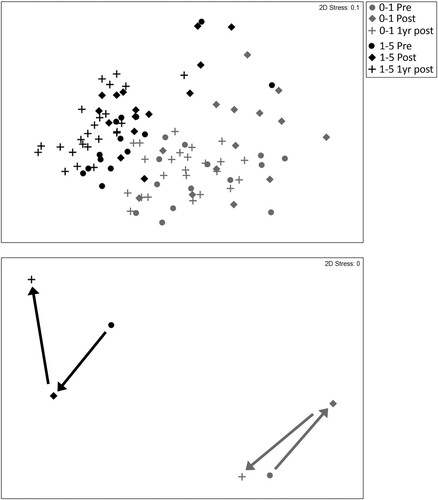
Table 8. Results of DistLM analyses showing correlations between environmental parameters and meiofauna community structure post-disturbance and 1 year post disturbance (combined directly and indirectly disturbed (DI) and undisturbed or indirectly disturbed sites (UI)). TOM = %total organic matter; C:N = molar carbon to nitrogen ratio in sediment organic matter (i.e. molar POC:PN); PN = %sediment particulate nitrogen; POC = %sediment particulate organic carbon; Silt/clay = %silt/clay; Chl a = sediment chlorophyll a in µg/g dry sediment; Phaeo = sediment phaeopigments in µg/g dry sediment.

	Pseudo-F	P	Prop
0-1 cm
Marginal tests
TOM	5.625	0.001	0.14
C:N	3.057	0.034	0.08
Porosity	2.637	0.046	0.07
Sequential tests
TOM	5.625	0.001	0.14
1-5 cm
Marginal tests
Chl a	3.326	0.040	0.09
Phaeo	2.916	0.043	0.08
C:N	3.117	0.038	0.08
Silt/clay	3.161	0.035	0.09
Sorting	2.508	0.073	0.07
Sequential tests
Chl a	3.326	0.032	0.09

Nodder SD, Eager C, O’Callaghan J, Leduc D, Deppeler S, Gerring P, Searson S, Quinn W, George S, Overden R, et al. in prep. Near-bed sediment dynamics and fluxes within the Subtropical Frontal Zone on Chatham Rise crest, and implications for deep-sea bottom trawling and seabed mining.

 Google Scholar

Clark MR, Nodder S, O'Callaghan J, Browne R, Daymond A, de Joux P, George S, Hale R, Hart A, Jhugroo K, et al. 2019. Resilience of deep-sea benthic communities to the effects of sedimentation (“ROBES”): Voyage report of Survey 2: June 2019. NIWA Client Report 2019330WN.

 Google Scholar