Figures & data
Figure 1. Modelled magnetic (a) and electric (b) field distributions of the single-turn coil with a magnetic core located in the x-y plane at z = −1.55cm. (c) Magnetic field strength along x, at y = 0, for various z values. The transition between bimodal and unimodal behaviour occurs at z ≈ 2. (d) Cross-sectional diagram of the experimental setup at y = 0 (i.e. vertically bisecting the phantom), drawn to scale and further described in the methods section.
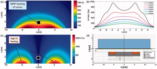
Figure 2. Modelled cross-sectional SAR distribution (xz-plane at y = 0) for a 0.6 S/m phantom with 1-cm3 uniformly distributed MNP inclusion. Regions of high EC SAR to be blocked by a tissue displacer are marked with dashed lines.
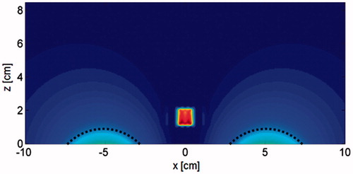
Figure 3. (a) AMF system with a phantom experiment in progress. The generator, treatment table, thermal camera, and thermal camera software interface are shown. (b) The induction coil is obscured from view in (a) by the treatment table.
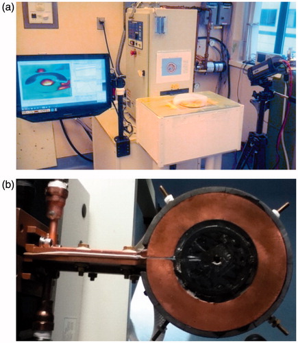
Figure 4. (a) A 2D cross-sectional diagram showing the geometry and relevant dimensions of the displacer. (b) 3D model of toroid section-shaped tissue displacer. (c) Cross-sectional diagram of the experimental set-up at y = 0 (drawn to scale).
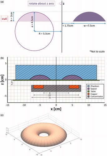
Figure 5. Top-down diagram of phantom positions during ECM-motion technique, note the phantom is positioned above the coil. (a) Coil position (copper coloured ring) shown with 12 positions for placement of the centre of the phantom. (b) Phantom (blue, dashed outline) in position 1, and (c) in position 2. Note that the phantom is simply translated to the next position and undergoes no rotation.
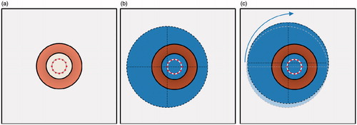
Figure 6. Modelled cross-sectional SAR distributions of control and displaced phantoms at z = 0, 2, and 4 cm (i.e. the base of the phantom, the height of the displacer, and 2 cm above the displacer).
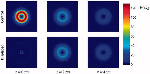
Figure 7. SAR distribution for control and displaced phantoms. Cross-sections shown at y = 0 cm.
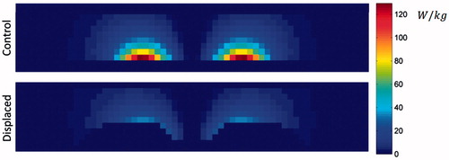
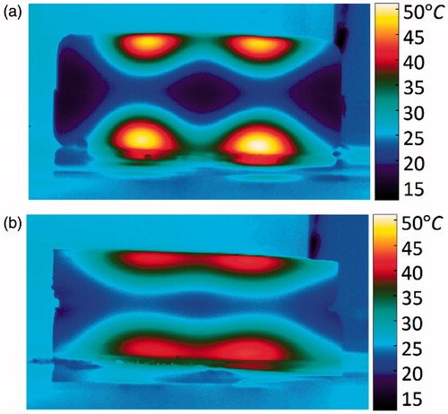
Figure 8. Resulting temperature distribution at various time points for the control phantom at z = 0 cm, and the displaced phantom at z = 2 cm. The cross-sections shown each contain the maximum temperature.
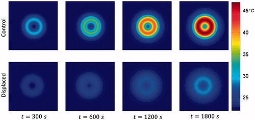
Figure 9. Resulting temperature distribution at t = 1800 s, y = 0 cm, for the control and displaced phantoms.
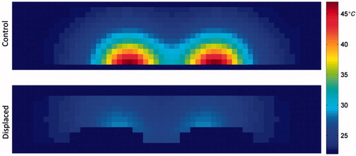
Figure 10. Position of bottom half of control phantom (a) and displaced phantom (b) after sectioning. Resulting cross-sectional temperature distributions at t = 1900 s for control (c) and displaced phantoms (d).
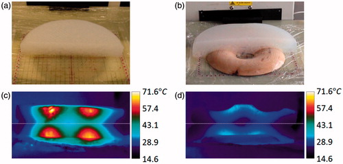
Figure 11. Diagram of phantom in (a) control position, i.e. centred over coil, (b) resulting SAR distribution of phantom in control position at z = 0 cm, (c) diagram of phantom in position 1 (x = −2.5 cm, y = 0 cm), (d) resulting SAR distribution of phantom at position 1, (cross-section shown at z = 0 cm).
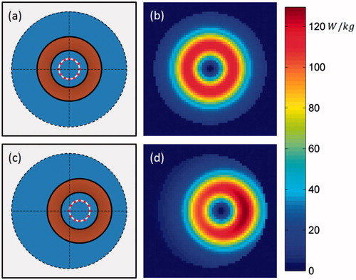
Figure 12. SAR distribution of the centred control phantom, and of the motion phantom at position 1. Cross sections shown at y = 0 cm.
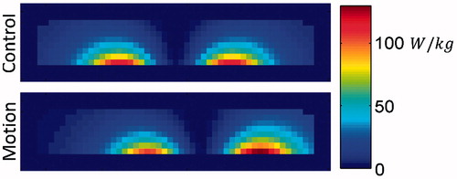
Figure 13. Resulting temperature distribution at the base of the phantom (z = 0 cm), for various time points, with the phantom in the control position (centred) throughout the exposure, and having moved between the 12 offset positions at 30-s intervals throughout the exposure.
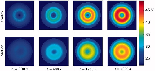
Figure 14. Resulting temperature distribution at t = 1800 s, with the phantom in the control position throughout the exposure, and having moved between the 12 offset positions at 30-s intervals throughout the exposure. Cross-sections shown in the xz-plane at y = 0 cm, i.e. bisecting the phantoms.
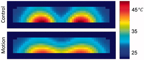
Figure 15. Resulting cross-sectional temperature distributions at t = 1890 s (90 s post-exposure) for (a) control and (b) motion phantoms.