
Figures & data
Figure 1. Schematic of the biophysical situation: breast cross section, tumour, tissue layers and the thermal boundary conditions.
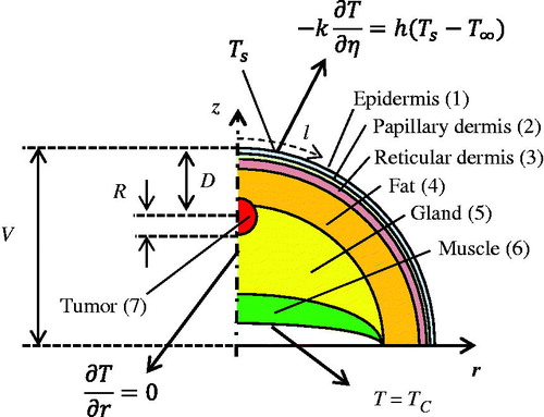
Table 1. Thermophysical properties of the tissue layers in Equation (1).
Figure 2. (a) Computational mesh, (b) computed temperature distribution in the cancerous breast and (c) coordinate system and surface data points used for the inverse reconstruction.
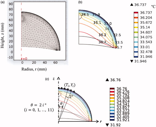
Figure 3. Flowchart of the inverse reconstruction algorithm.
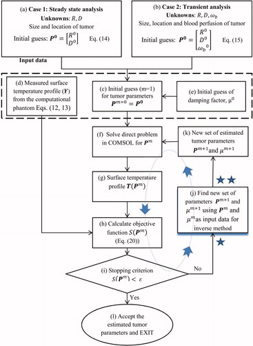
Figure 4. Flowchart describing block (j) in .
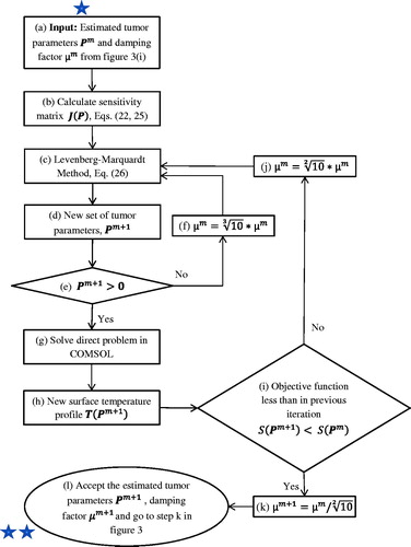
Figure 5. Temperature rise ΔT at a point directly above the tumour corresponding to θ0=0o as a function of tumour radius R and depth D for blood perfusion values (a) ωb= 0.003 m3/s/m3, (b) ωb= 0.006 m3/s/m3, (c) ωb= 0.009 m3/s/m3 and (d) ωb= 0.012 m3/s/m3.
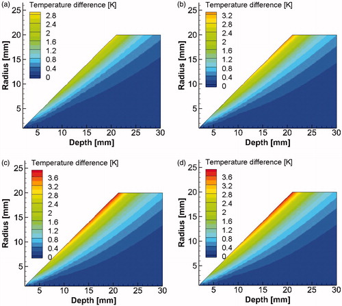
Figure 6. Evolution of (a) depth D and (b) radius R of the tumour and (c) error S(P) versus the iteration number using steady state data for the three cases in .
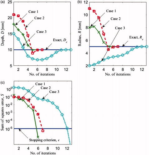
Table 2. Exact tumour parameters D and R and three sets of initial guesses (cases 1, 2 and 3) for the inverse problem with two unknowns (steady state analysis).
Figure 7. Evolution of (a) depth D (b) radius R (c) blood perfusion rate ωb of the tumour and the (d) error S(P) versus the number of iterations using steady state data for the three cases in .
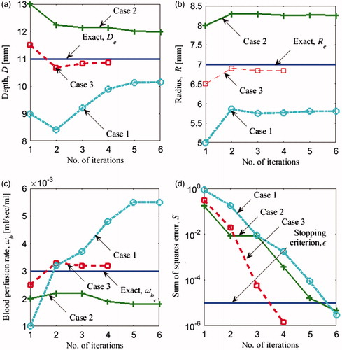
Table 3. Exact parameter values and three sets of initial guesses for the inverse problem with three unknowns for steady state analysis. Temperature rise for sets of parameters marked by * is plotted in .
Figure 8. Surface temperature profiles for tumour parameters marked by * in .
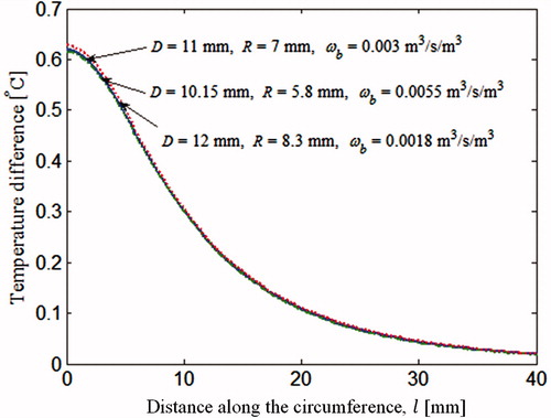
Figure 9. Thermal recovery temperature profile of a point directly above the tumour corresponding to θ0. The tumours considered are the 3 tumours marked by * in and are also discussed in .
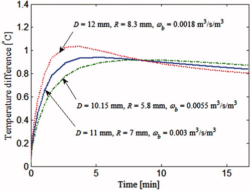
Figure 10. Evolution of (a) depth D (b) radius R (c) blood perfusion rate ωb of the tumour and (d) error S(P) versus the number of iterations using transient data for the three cases summarised in .
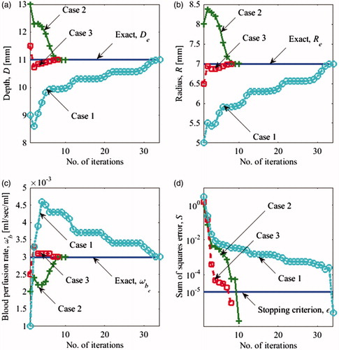
Table 4. Exact parameter values and three sets of initial guesses for the inverse problem with three unknowns for transient analysis.
Table 5. Exact parameter values and sets of initial guesses for the inverse problem with three unknowns for transient analysis.
Table 6. Exact parameter values and sets of initial guesses for the inverse problem with three unknowns for transient analysis. A 10 mK noise was added to the surface temperature and a stopping criterion ɛ = 5 * 10−4 was used.