Noninvasive intratumoral thermal dose determination during in vivo magnetic nanoparticle hyperthermia: combining surface temperature measurements and computer simulations

Figures & data

Figure 1. (A) Schematic representation of MalbIR nanocarrier. (B) Molecular structure of the IR-780 generated using the free-license software Pymol to estimate the size of the molecule, where the unit of measurement is in angstrom (1 Å=10⁻¹⁰ m). (C) Representative HR-TEM image of the Mn-ferrite nanoparticles (with diameter $\sim$13 nm). (D) MalbIR nanocarrier size distribution obtained from NTA analysis. (E) Representative FE-SEM image of the MalbIR nanocarrier.

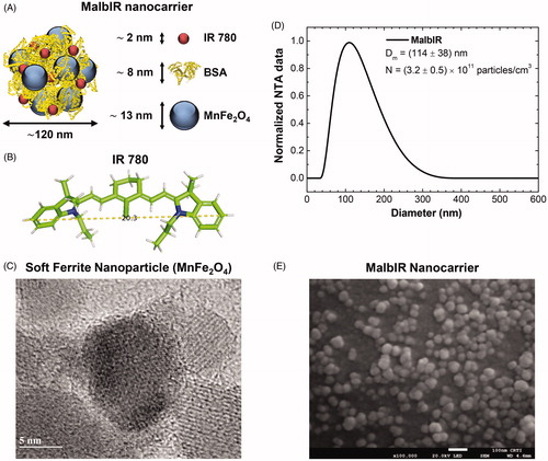
Figure 2. (A) Tumoral time-evolution of the control group (n = 5), animals also bearing a solid and subcutaneous Ehrlich tumor, that did not undergo the MNH nor receive MalbIR injection. (B) Tumoral time-evolution of the treated animals #2, #3 and #4 by in vivo MNH with MalbIR nanocarriers intratumoral injection (single session of 30 min of exposure to an AMF of 17.5 kA.m⁻¹ and 301 kHz). (B) Kaplan–Meier’s curves of the control group (in black, they were euthanized when their tumors reached 2000 mm³) and the treated animals #2, #3 and #4 (in red). (C) Histological sections of the skin of animal #3, extracted from the same region where the tumor had previously been induced, but 575 days after the MNH treatment. The red arrows indicate fibrotic regions and the black arrows indicate the dermis and muscle tissue.

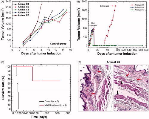
Figure 3. Animal’s body reconstruction: (A) picture of animal #1 (before MNH) sedated and positioned in the same way that it will be placed inside the coil for treatment; (B) diagram illustrating the process to take sequential pictures of this animal's body collecting a close-range photographic data set with the digital camera; (C) animal’s body model reconstructed by photogrammetry technique. Animal’s tumor volume reconstruction: (D) ultrasonography showing the animal in the prone position, identifying its solid tumor along the vertebral column (dorsal region); (E) process for tumor slice extraction from the ultrasound video (about 100 frames) and filter applications to the images; (F) rendering of the tumor volume after stacking all the filtered slices. Nano-heaters intratumoral spatial distribution: (G) 3D animal scanning on the fluorescence molecular tomography (FMT); (H) 3D reconstruction of the volume occupied by the MalbIR nanocarriers within the tumoral mass (less than 1 h after intratumoral injection); (I) three-dimensional heat source distribution function (voxel-dependent) generated using the COMSOL Multiphysics software.

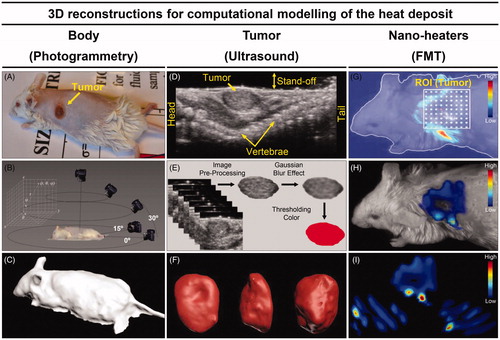
Figure 4. (A) Thermographic image of animal #1 at time t = 31 min (i.e., after 30 min of MNH). (B) It is a pixelated IR image from the ROI_Tumor enclosing a total amount of 750 pixels (where each one of them works like a punctual thermometer). (C) The numerically calculated temperature compared to the real value (IR measurement) at the same point of the mouse skin surface. (D) (I, II) Customized meshes generated using COMSOL Multiphysics commercial software for the application of the finite element method of calculation within the animal’s body and tumor reconstructed geometries (animal #1); (III) the volumetric distribution of the heat-sources, inside the animal’s tumor #1, based on the 3D-FMT mapping of the MalbIR nanocarriers. (E) (IV) shows the numerical calculation of the mouse skin surface temperature (all over the body), after 30 min of MNH; (V) ROI_Tumor extracted from the simulation showing the temperature profile after 30 min of MNH.

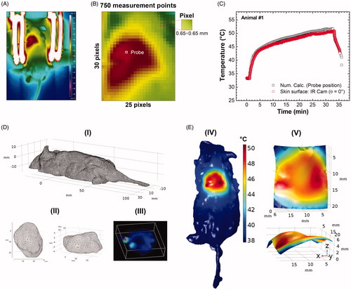
Figure 5. (A) Tumoral evolution of animal #1 until the MNH treatment day (about 738 mm³): the animal #1 was euthanized on the 11th day and the excised tumor tissue was used for a histopathologic assay (positive control). (B) Histopathological slide with three parts of the tumor excised from animal #1. The red arrows indicate the portions of skin and muscle that was not properly removed during the tumor excision (overestimating total tumoral tissue region). This skin and muscle layers have been computationally removed from this slice (the inset on image). (C) The threshold color method option is applied to delimit apoptotic/necrotic (red) and viable (black) areas. This process is done for all images in the stack (∼110 slices). (D) The animal’s #1 skin temperature data within the experimental (4 D-I) and simulated (D, II) ROI_Tumor, at time instant t = 31 min, i.e., after 30 min of MNH. Each temperature map contains 750 pixels. (D, III) shows the temperature difference (T_Sim – T_IR), pixel by pixel, between the simulated and the experimental ROI_Tumor. When |T_Sim – T_IR|≤1 °C both pixels are considered registering the same temperature value (due to the IR measurements experimental error ± 1 °C). From this, it is possible to estimate the percentage of area agreement between experimental (D, I) and simulated (D, II) data. (E) Pixel agreement curve as a function of SLP_sim for animal #1, using the Erdmann model. (F) The upper part (red solid) shows the simulated fraction, within the total tumor #1, of the tissue volume irreversibly damaged (V_IrrevDam=550 mm³) and, in the lower part (blue solid), the simulated fraction that has suffered reversible thermal damages and remains viable (V_RevDam=188 mm³), when ${\theta }_c=0.75.$

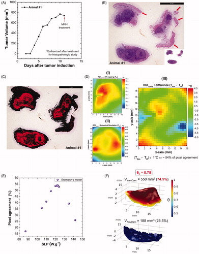
Figure 6. (A) Calculated fraction of irreversible tumor lesion (%) (after 30 min of MNH) as a function of SLP for the different tumor blood perfusion expressions (see Table S-III). (B) Surface area pixel agreement (inside ROI_Tumor), between the IR data and the numerically calculated values for animal's skin temperature after 30 min of MNH, for several perfusion cases. (C) The calculated fraction of irreversible tumor lesion (%) (after 30 min of MNH) as a function of SLP, for different $h$ values assuming Erdmann’s model (Equation (5)) for the perfusion (shown in the inset). (D) Surface area pixel agreement as a function of SLP, at 30 min of MNH, for the same $h$ values tested in (C) and also assuming Erdmann’s model.

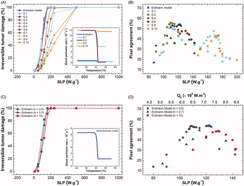
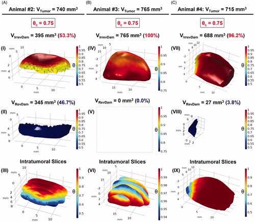
Figure 7. Volumetric fractions of irreversibly damaged (in red) and viable tissues (in blue) were numerically calculated for the tumoral volumes of animals #2, #3 and #4, columns A, B and C, respectively, assuming Erdmann’s perfusion model (Equation (5)). (A) In (I) the irreversible thermal damage value was calculated, corresponding to a volume of 395 mm³ of the total volume of animal #2 (740 mm³). The reversible thermal damage (II) is obtained by putting the volume to which ${\theta }_c<0.75$ is blue. (III) The intratumoral slices allow an internal visualization of the distribution of the degree of tissue injury of the tumor. The same analysis was done for animal #3 (B) and #4 (C). In (IV), ${\theta }_c=0.75$ was adopted and the value of 765 mm³ was obtained for the volume of irreversible thermal damage, that is, 100% of the degree of tissue injury. This means that there is no viable tumor volume in (V), so it is blank. Intratumoral slices show the intratumoral tissue lesion in (VI), the scale shows that there are no ${\theta }_c<0.75,$ consistent with the results of (V). It is easy to notice the difference between the necrotic volumes between animals #2 and #4. By analyzing the number of data from COMSOL, animal #2 had irreversible thermal damage in only 53.3%. For animal #4, the irreversible volume was 688 mm³, equivalent to 96.2%.