In silico assessment of collateral eddy current heating in biocompatible implants subjected to magnetic hyperthermia treatments

Figures & data

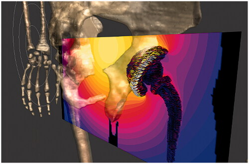
Figure 1. (i) Virtual models used for each of the considered cases, indicating the position of prostheses and coils (white hairlines): (a) head-and-neck, (b) colorectal, (c) prostate, and (d) worst-case scenario tumor locations. For (a) a 3-turn open collar-type coil has been considered, while for (b), (c) and (d) a 3-turn (inner turn of 5 cm, intermediate turn 10 cm, and outer turn of 15 cm) non-spiral, single layer, flat air coil has been used instead. For comparison purposes, prostheses are made of either Ti6Al4V or CoCrMo alloys in all the indications. (ii) Portion of voxels in the surrounding of each prosthesis that are taken into account for the scatter plot analysis. (iii) Detail of the coil used for CR, Pr and WCS tumor locations. Dimensions are presented in mm. (iv) Detail of the coil used for NH tumor location. Dimensions are presented in mm.

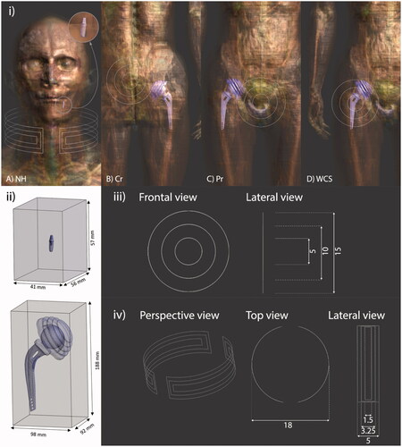
Table 1. Electrical and thermal properties of the implant materials used in the simulations.

Material	$\sigma \mathrm{ }(\mathrm{kS}/\mathrm{m})$	$\rho \mathrm{ }(\mathrm{kg}/{\mathrm{m}}^3)$	$c_p\mathrm{ }(\mathrm{J}/(\mathrm{kg}·\mathrm{K}))$	$\lambda (\mathrm{W}/(\mathrm{m}·\mathrm{K}))$
Ti6Al4V [55]	560	4430	526.3	6.7
Metal-ceramic [56,57]	0.16	8400	450	13
CoCrMo [57]	1160	8400	450	13

Figure 2. Log-log scatter plots of ΔT versus SAR for bone voxels at f = 300 kHz with magnetic flux density of 15 mT without accounting for thermoregulation. The figures in the right column refer to colon tumor, the one in the left column to prostate tumor. Color varies depending on the distance of each voxel to its closest point in the coil (reddish points are closer to the coil and bluish points are farther from it). The thresholds are established according to ICNIRP 2020 guidelines for type 1 tissues, namely ΔT = 5 °C and SAR = 10 W/kg.

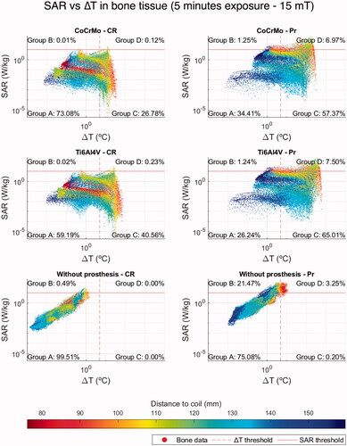
Table 2. Percentage of bone tissue voxels that land in each quadrant for fields of 5, 10 and 15 mT in the tumor region for each case for both 5- and 30-min exposure.

		5 min exposure					30 min exposure
		Quadrant				Risk	Quadrant
		A	B	C	D		A	B	C	D	Risk
5 mT	CR CoCrMo	100.00%	0.00%	0.00%	0.00%	0.06 (S)	99.21%	0.00%	0.79%	0.00%	0.06 (S)
	CR Ti6Al4V	99.27%	0.00%	0.73%	0.00%	0.06 (S)	95.58%	0.00%	4.42%	0.00%	0.07 (S)
	CR without prosthesis	100.00%	0.00%	0.00%	0.00%	0.06 (S)	100.00%	0.00%	0.00%	0.00%	0.06 (S)
	Pr CoCrMo	78.61%	0.00%	21.17%	0.22%	0.14 (A)	71.69%	0.00%	28.09%	0.22%	0.17 (R)
	Pr Ti6Al4V	82.11%	0.00%	17.63%	0.26%	0.13 (A)	Out of range	Out of range	Out of range	Out of range	Out of range
	Pr without prosthesis	99.99%	0.01%	0.00%	0.00%	0.06 (S)	99.99%	0.01%	0.00%	0.00%	0.06 (S)
10 mT	CR CoCrMo	90.15%	0.00%	9.84%	0.00%	0.09 (S)	80.68%	0.00%	19.31%	0.00%	0.13 (A)
	CR Ti6Al4V	82.03%	0.00%	17.95%	0.02%	0.13 (A)	75.89%	0.00%	24.09%	0.02%	0.15 (R)
	CR without prosthesis	99.94%	0.06%	0.00%	0.00%	0.06 (S)	99.94%	0.06%	0.00%	0.00%	0.06 (S)
	Pr CoCrMo	Out of range	Out of range	Out of range	Out of range	Out of range	Out of range	Out of range	Out of range	Out of range	Out of range
	Pr Ti6Al4V	Out of range	Out of range	Out of range	Out of range	Out of range	Out of range	Out of range	Out of range	Out of range	Out of range
	Pr without prosthesis	87.73%	12.27%	0.00%	0.00%	0.06 (S)	87.73%	12.27%	0.00%	0.00%	0.06 (S)
15 mT	CR CoCrMo	75.60%	0.02%	24.25%	0.14%	0.15 (R)	67.71%	0.02%	32.13%	0.14%	0.18 (R)
	CR Ti6Al4V	68.73%	0.04%	30.99%	0.25%	0.18 (R)	63.29%	0.04%	36.43%	0.25%	0.20 (R)
	CR without prosthesis	99.47%	0.53%	0.00%	0.00%	0.06 (S)	99.47%	0.53%	0.00%	0.00%	0.06 (S)
	Pr CoCrMo	Out of range	Out of range	Out of range	Out of range	Out of range	Out of range	Out of range	Out of range	Out of range	Out of range
	Pr Ti6Al4V	Out of range	Out of range	Out of range	Out of range	Out of range	Out of range	Out of range	Out of range	Out of range	Out of range
	Pr without prosthesis	Out of range	Out of range	Out of range	Out of range	Out of range	Out of range	Out of range	Out of range	Out of range	Out of range

Risk column color indicates the safety of each case according to Equation (5)(5) $$\text{risk index}=0.0555·\mathrm{A}+0.1165·\mathrm{B}+0.4439·\mathrm{C}+0.5199·\mathrm{D},$$(5) , the darker, the riskier; and a letter that indicates the risk: (S), safe; (A), acceptable; (R), risky; (VR), very risky. Note that results presented for Pr Ti6AlV at 5 mT shown in bold italics are after 2 min exposure instead of 5. This corresponds to the last instant the thermoregulation model retrieves.

Figure 3. Different views of the 3 D scatter plot of the magnetic flux density through the prosthesis voxels, the increment of temperature for these voxels and the closest distance to the coil for the three cases studied: (a) 3 D view, (b) XY view, (c) XZ view, and (d) YZ view.

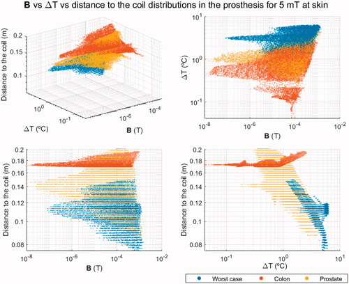
Figure 4. Log-log scatter plots representing the ΔT and SAR of bone voxels for a dental implant studied with and without the metal-ceramic crown attached to it both exposed for 30 min to the same applied ac field with f = 300 kHz and 15 mT. The thresholds are established according to ICNIRP 2020 guidelines for type 1 tissues, namely ΔT = 5 °C and SAR = 10 W/kg.

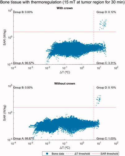
Table 3. Percentage of bone tissue voxels that fall within each quadrant in Figures 4, Supplementary Figures S5 and S6 plots.

				Quadrant				Risk
				A	B	C	D
With thermoregulation	5 min exposure	5 mT	With crown	99.90%	0.10%	0.00%	0.00%	0.06 (S)
			Without crown	99.92%	0.08%	0.00%	0.00%	0.06 (S)
		10 mT	With crown	98.83%	0.00%	1.05%	0.12%	0.06 (S)
			Without crown	99.88%	0.04%	0.02%	0.06%	0.06 (S)
		15 mT	With crown	97.03%	0.00%	2.85%	0.12%	0.07 (S)
			Without crown	98.95%	0.00%	0.95%	0.10%	0.06 (S)
	30 min exposure	5 mT	With crown	99.99%	0.01%	0.00%	0.00%	0.06 (S)
			Without crown	99.99%	0.01%	0.00%	0.00%	0.06 (S)
		10 mT	With crown	98.62%	0.00%	1.26%	0.12%	0.06 (S)
			Without crown	99.86%	0.03%	0.04%	0.06%	0.06 (S)
		15 mT	With crown	96.57%	0.00%	3.31%	0.12%	0.07 (S)
			Without crown	98.87%	0.00%	1.03%	0.10%	0.06 (S)
Without thermoregulation	5 min exposure	5 mT	With crown	99.90%	0.10%	0.00%	0.00%	0.06 (S)
			Without crown	99.92%	0.08%	0.00%	0.00%	0.06 (S)
		10 mT	With crown	96.91%	0.00%	2.97%	0.12%	0.07 (S)
			Without crown	99.65%	0.02%	0.26%	0.07%	0.06 (S)
		15 mT	With crown	91.86%	0.00%	8.02%	0.12%	0.09 (S)
			Without crown	97.40%	0.00%	2.51%	0.10%	0.07 (S)

Risk column color indicates the safety of each case according to expression (5), the darker, the riskier; and a letter that indicates the risk: (S), safe; (A), acceptable; (R), risky; (VR), very risky.

Figure 5. Slice Z normal views: (a) of the effective magnetic field for the worst-case scenario with and without prosthesis for an ac field with 5 mT at skin level; and (b) of the difference between effective magnetic field for the worst-case scenario with and without Ti6Al4V prosthesis. The alteration due to the generated field drops to values around 0.1 mT for distances below 1 cm away from the implant.

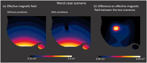
Figure 6. (a) ΔT evolution over time for the three considered field intensities (5, 10 and 15 mT), for the same indication (colon cancer case), and the same prosthesis type (Ti6Al4V hip implant). Each curve tracks the temperature evolution for (i) the first voxel in surpassing the ICNIRP ΔT threshold, (ii) the global maximum of ΔT in tissue at all times, and (iii) the globalmaximum of ΔT in the prosthesis at all times. (b) ΔT evolution over time for the two prosthesis materials considered (Ti6Al4V and CoCrMo), for the same indication (colon cancer case), under the same field conditions (15 mT, 300 kHz). Each curve tracks the temperature evolution for (i) the first voxel in surpassing the ICNIRP ΔT threshold, (ii) the global maximum of ΔT in tissue at all times, and (iii) the global maximum of ΔT in the prosthesis at all times.

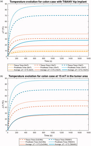
Table 4. Main parameters from the curves featured in Figure 6 (threshold ΔT = 5 °C, maximum temperature in tissue, and maximum temperature in prosthesis).

	Time (s)
	Figure 6(a) (Ti6Al4V)			Figure 6(b) (15 mT)
Parameter	5 mT	10 mT	15 mT	Ti6Al4V	CoCrMo
Threshold ΔT = 5 °C	540	690	930	930	1020
Maximum temperature in tissue	540	690	870	870	990
Maximum temperature in prosthesis	570	720	900	900	1020

The reported time values are those so that the derivative of the temperature vs time curves is less than 0.001 s.

http://www.matweb.com/search/datasheet.aspx?MatGUID=a0655d261898456b958e5f825ae85390 [accessed 2021 Apr 6].

 Google Scholar

Tanaka Y, Saito H, Tsutsumi Y, et al. Active hydroxyl groups on surface oxide film of titanium, 316L stainless steel, and cobalt-chromium-molybdenum alloy and its effect on the immobilization of poly(ethylene glycol). Mater Trans. 2008;49:805–811.

 Web of Science ®Google Scholar

Starčuková J, Starčuk Z, Hubálková H, et al. Magnetic susceptibility and electrical conductivity of metallic dental materials and their impact on MR imaging artifacts. Dent Mater. 2008;24:715–723.

 PubMed Web of Science ®Google Scholar

Data availability statement

The whole dataset obtained during the course of this study is publicly available for download. The files are uploaded in the Zenodo repository under the title ‘Dataset from “In silico assessment of collateral eddy current heating in biocompatible implants subjected to magnetic hyperthermia treatments”.’ The structure of the files is also explained [66].