In-beam PET measurements of biological half-lives of ¹²C irradiation induced β⁺-activity

Figures & data

Figure 1.  Double head positron camera at the treatment site at GSI Darmstadt, Germany. The red arrow denotes the beam direction.

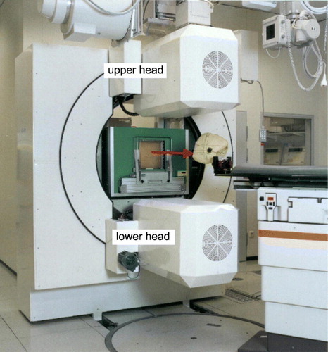
Figure 2.  Time-event-histogram of a patient irradiation. During the particular irradiation shown the beam delivery starts with the lowest energy necessary for irradiating the tumour. The energy is increased stepwise until the particles reach the distal edge of the tumour. The beam delivery was interrupted by about 1 minute (dash-dotted lines) due to technical reasons. The rectangular graph in the inset denotes the beam extraction from the synchrotron, high value means beam extraction, low value extraction pause. The information on the status of the beam was also stored in the data stream. The annihilation events registered during beam extraction are rejected from further processing, since they are massively corrupted by random coincidences from prompt γ-rays following nuclear reactions between the projectiles and the atomic nuclei of the target [2], [13], [14]. The dotted line indicates the end of the irradiation and the beginning of the 40 s decay measurement.

Figure 3.  β⁺-activity depth profiles in different targets obtained by using back projection. The red lines display the activity measured during the irradiation, the blue dashed lines give the activity measured between 10 and 20 min after the end of the irradiation. The red curve was normalised to the maximum of the measured β⁺-activity during the irradiation and the blue curve was scaled according to this. The peak at the distal end arises from long-lived projectile fragments such as ¹¹C. Target fragments were produced along the whole beam path. The lower row shows the location of the ROI (1) and ROI (2) for separating the coincidences from target (1) and projectile (2) fragments, respectively.

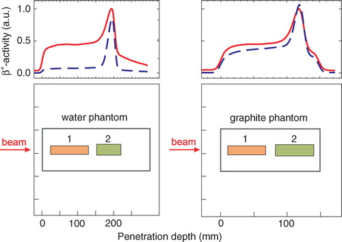
Figure 4.  Effective half-lives T_1/2^{(eff, phys)} as a function of the decay time t_d. All measured true coincidences were used for the fit. The effective half-life of human tissue was calculated as weighted mean of the half-lives of the graphite and water target.

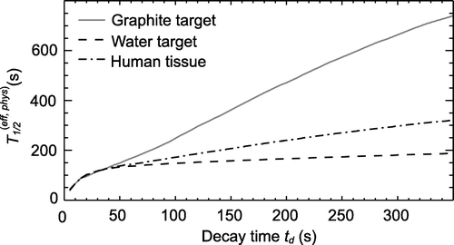
Table I.  Effective half-lives T_1/2^{(eff, phys)} in the phantoms analysing different spatial subsets of the data as a function of the decay time t_d after finishing the irradiation. The regions are defined according to Figure 3. The error is two times the standard deviation of the fitted parameter. If the ROI is referred to as ‘phantom’ all data were used for that fit.

Target material	ROI	T1/2^(eff, ^phys)/s (td=40 s)	T1/2^(eff, ^phys)/s (td=300 s)
water	1	143±6	162±1
water	2	135±6	242±1
water	phantom	127±3	180±1
graphite	1	152±14	748±19
graphite	2	147±10	716±13
graphite	phantom	131±5	663±7

Figure 5.  Two-dimensional histogram for the fraction of the LOR intersecting the irradiated volume as a function of HU_mean and σ_HU. The corresponding anatomical regions for a particular patient can be seen in Figure 6.

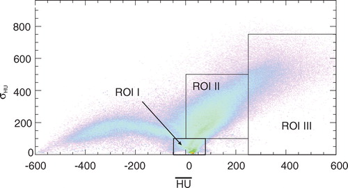
Figure 6.  Effective half-lives in the patient and the back projections of the used coincidences according to the regions defined in Figure 5 to outline the corresponding anatomical regions. The left figure corresponds to ROI I, the middle one to ROI II and the right one to ROI III, respectively.

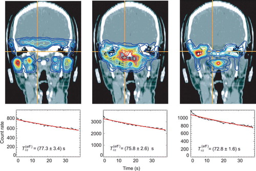
Figure 7.  β⁺-activity distributions superimposed onto a patient CT. (1) shows the measurement, (2) simulation without considering the washout, (3) simulation with a weighted mean of T_1/2^(biol), (4) a dose dependent T_1/2^(biol) was used. The circles are to guide the eyes where an improvement of the simulation over a biological half life is obvious.

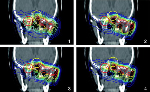
Figure 8.  β⁺-activity distributions superimposed onto a patient CT. (1) shows the measurement, (2) simulation without considering the washout, (3) simulation with a weighted mean of T_1/2^(biol), (4) a dose dependent T_1/2^(biol) was used. The solid line shows the range, which is reproduced much better in the simulations considering the washout, the circles are to guide the eyes where an improvement of the simulation over a biological half life is obvious.

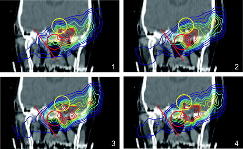
Table II.  Effective half-lives as a function of the HU_mean and σ_HU as outlined in Figure 5. The error is two times the standard deviation of the fitted parameter.

ROI	Range HUmean	σHU	T1/2^(eff)/s
I	−50 < HU < 75	0 < σ < 100	77.3±3.4
II	0 < HU < 250	100 < σ < 500	75.8±2.6
III	250 < HU < 600	0 < σ < 750	72.8±1.6

Table III.  Effective half-lives estimated from the patient data and biological half-lives calculated according to the formula given in section “Extraction of the effective half-lives” in dependence on the dose. The error is two times the standard deviation of the fitted parameter.

Dose range /%	T1/2^(eff)/s	T1/2^(biol)/s
0–100	73.2±0.5	170.8±8.6
0–50	72.8±1.1	168.6±11.6
0–90	71.8±0.6	163.2±8.5
50–100	73.8±0.7	174.1±9.4
90–100	79.5±1.8	209.5±21.3

Figure 9.  Influence of the treatment time on the effective half-life as a function of the dose. In the upper line, the back projected coincidences emerging from the regions which meet the conditions are displayed as an example. The left side shows the dose range 0–90%, the right side that for 90–100% and the diagrams in the lower line give the decrease of the effective half-life during the treatment.

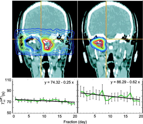
Table IV.  The rise of the fit of the effective half-life as a function of the treatment time. The given error is two times the uncertainty for the fit parameter.

Dose range /%	Change of the effective half-life (s/fraction)
0–100	−0.34±0.15
0–50	−0.20±0.20
0–90	−0.25±0.16
50–100	−0.39±0.19
90–100	−0.62±0.37

Enghardt W, Crespo P, Fiedler F, Hinz R, Parodi K, Pawelke J, et al. Charged hadron tumour therapy monitoring by means of PET. Nucl Instr Meth A 2004; 525: 284–8

 Web of Science ®Google Scholar

Parodi K, Crespo P, Eickhoff H, Haberer T, Pawelke J, Schardt D, et al. Random coincidences during in-beam PET measurements at microbunched therapeutic ion beams. Nucl Instr Meth A 2005; 545: 446–58

 Web of Science ®Google Scholar

Crespo P, Barthel T, Frais-Kölbl H, Griesmayer E, Heidel K, Parodi K, et al. Suppression of random coincidences during in-beam PET measurements at ion beam radiotherapy facilities. IEEE Trans Nucl Sci 2005; 52: 980–7

 Web of Science ®Google Scholar