Systematic trends in the substitution mechanisms of minor elements in cassiterite

Figures & data

Table 1. A selected summary of minimum Sn contents, and maximum concentrations of substituting elements measured by EPMA, as reported in the literature from different localities. The number of decimal places reflect the reported precision from the original source. All values converted to apfu*100, based on 2 atoms of oxygen per 1 cation. Not all values belong to the same analytical point, or even crystal, and totals will not equal 100. <dl = below the limit of detection, - = not analysed.

Reference, locality	System	Element concentration (in apfu*100)										Other trace
		Sn	Al	Si	Ti	Mn	Fe	Zr	Nb	Ta	W
Hall and Ribbe, 1971
Numerous Localities^a	Mixed^a	<93^b	4.70	3.40	3.5	0.66	6.74	–	5.31	3.81	0.69	S: 0.14
Moore and Howie, 1979
Cligga Head, Cornwall, UK	Quartz Vein	97.23	–	1.08	0.11	–	1.31	–	0.29	0.02	1.04	In: 0.05; Ir: 0.01
St. Michael’s Mount, Cornwall, UK	Quartz Vein	98.65	–	0.90	0.15	–	0.60	–	0.11	0.06	0.05	In: 0.05; Ir: 0.01
Izoret et al., 1985
Fontao, Gallicia, Spain	Greisen	94.63	–	–	2.19	–	1.63	–	2.68	2.75	–
Santa Comba, Gallicia, Spain	Quartz Vein	98.11	–	–	1.39	–	0.39	–	0.33	<dl	–
Monteneme, Gallicia, Spain	Quartz Vein	98.16	–	–	1.70	–	0.25	–	0.17	<dl	–
Penauta, Gallicia, Spain	Quartz Vein	93.93	–	–	2.06	–	2.04	–	1.18	2.39	–
Unspecified, Cornwall, UK	Quartz Vein	97.98	–	–	2.02	–	0.14	–	0.57	<dl	–
Farmer et al., 1991^c
South Crofty Mine, Cornwall, UK	Quartz Vein	98	–	–	1.09	–	0.91	–	–	–	0.26
Masau et al., 2000^d
Annie Claim #3, Manitoba, Canada	Pegmatite	91.10	–	–	0.10	2.40	1.80	0.30	0.90	5.00	0.20	As, Sb, Mg, Ca, Pb: 0.10; Hf, Th, U, Sc, Bi, Zn: <dl
Černý et al., 2004
Varuträsk, Sweden	Pegmatite	93.2	–	–	0.40	0.75	0.09	0.15	1.05	3.75	0.15	Zn: 0.15; As, Sb: 0.1; Ca, Bi, Pb: 0.05; Th, U: <dl
Pal et al., 2007
Govindpal	Pegmatite	91.2	–	–	<dl	1.30	1.30	–	0.60	5.40	<0.1
Mundaguda	Pegmatite	92.6	–	–	<dl	2.00	0.10	–	0.70	4.50	0.1
Dhuramagurah	Pegmatite	90.4	–	–	<dl	0.20	3.00	–	1.00	5.40	<dl
Bacheli	Pegmatite	92.1	–	–	<dl	0.20	2.10	–	2.00	3.40	<dl
Neiva, 2008
Argozelo	Quartz Vein	95.0	–	–	0.80	0.20	1.9	–	1.3	1.3	<dl
Carris	Quartz Vein	98.7	–	–	1.00	<dl	<dl	–	<dl	<dl	0.20
Filharoso	Quartz Vein	98.5	–	–	1.00	<dl	0.20	–	0.1	0.20	<dl
Vale das Gatas	Quartz Vein	98.8	–	–	1.10	0.20	0.10	–	<dl	<dl	<dl
Panasqueira	Quartz Vein	98.8	–	–	1.00	<dl	0.10	–	<dl	<dl	<dl
Caravalhal	Quartz Vein	98.0	–	–	1.40	0.10	<dl	–	<dl	<dl	<dl
Galliski et al., 2008
La Viquita	Pegmatite	84.5	–	–	<0.01	0.50	5.00	0.5	1.00	9.00	<dl	As, Sb, Bi, Mg, Ca, Zn, Pb, Th, U: <dl
Nambaje et al., 2020
Karagwe Ankole Belt, Rwanda	Quartz Vein	98.6	0.1	0.9	0.6	0.1	0.3	–	0.3	0.2	–	Mg, Zn: 0.2

a). Analyses of 40 samples from ∼25 localities, some unknown. Further details available in Hall, 1968. b). Total Sn contents are not reported, minimum Sn concentrations thus estimated from sum of ‘mean’ analyses. c). Values approximate, estimated from partial data. d). The appreciable presence of Hf in exsolved wodginite–ferrowodginite implies uptake in the primary cassiterite at levels below the sensitivity of EPMA.

Figure 1. A schematic illustration of the physicochemical model of cassiterite mineral systems employed in this study. Silicate Liquid Systems, where cassiterite precipitates from a silicate liquid, include (a) pegmatite deposits, and (b) granite-hosted Disseminated Sn deposits. Hybrid Systems, where cassiterite may precipitate from both silicate liquids and aqueous fluids, are represented by (c) greisen deposits. Aqueous Fluid Systems, where cassiterite is precipitated from hydrothermal fluids only, are represented by (d) vein-hosted systems and (e) Sn-bearing skarn systems. In this model, the key distinction between vein-hosted and skarn systems is the degree of wall-rock alteration (metasomatism), with vein-hosted systems representing a low alteration endmember, and skarn systems representing a high alteration endmember. The classification of cassiterite crystals examined in this study is also listed in this figure.

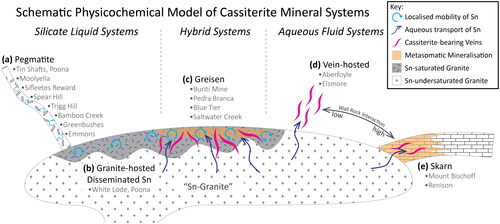
Table 2. Summary of the cassiterite samples and their localities used in this study, with approximate coordinates (accurate to within ±1 of the decimal place given). Each locality is classified into one of the simplified cassiterite mineral systems as outlined in Figure 1. Any coexisting mineral phases noted by previous authors are shown along with any classifications of each deposit type, for comparison (Paragenesis), taken from the key references for each locality. The nature of the samples used in this study, and any other notable characteristics, are described in Sample Observations and Characteristics.

Paragenesis/Locality (Latitude, Longitude)	References	Sample observations and characteristics
Granite-hosted disseminated Sn deposits
White Lode, Poona, Western Australia, Australia (–27.13°, 117.46°)
Kaolinised granite	Bennett et al., 2020; Grundmann & Morteani, 1998; Jacobson et al., 2007; Marshall et al., 2016	1–2 mm anhedral to euhedral cassiterite crystals disseminated in a kaolinite (after feldspar) quartz granitic matrix.
Pegmatite-hosted Sn deposits
Tin Shafts, Poona, Western Australia, Australia (–27.14°, 117.46°)
Lepidolite, cassiterite, columbite–tantalite, fluorite, garnet and apatite bearing pegmatite	Grundmann & Morteani, 1998; Jacobson et al., 2007; Marshall et al., 2016	∼5 mm anhedral crystal, collected loose from around the entrance to the shaft.
Moolyella, Western Australia, Australia (–21.14°, 119.89°)
Cassiterite, columbite–tantalite and magnetite bearing pegmatites	Jacobson et al., 2007	∼5 mm rounded eluvial crystal.
Sifleetes Reward, Western Australia, Australia (–21.27°, 118.61°)
Cassiterite, columbite, lepidolite, tourmaline and topaz bearing pegmatite	Jacobson et al., 2007	3 × 2 mm rectangular crystal in quartz–feldspar–mica pegmatitic matrix.
Spear Hill, Western Australia, Australia (–21.51°, 119.42°)
Cassiterite bearing pegmatites	Jacobson et al., 2007	∼10 mm sub-angular eluvial crystal.
Trigg Hill, Western Australia, Australia (–21.60°, 119.29°)
Cassiterite, monazite and tanteuxenite bearing microcline–quartz pegmatites	Jacobson et al., 2007; Sweetapple & Collins, 2002	2–3 mm rounded eluvial cassiterite crystals.
Greenbushes, Western Australia, Australia (–33.86°, 116.06°)
Cassiterite, tantalite, albite and spodumene bearing Sn–Ta–Li pegmatite	Partington et al., 1995	∼1 mm rounded eluvial crystal.
Bamboo Creek, Northern Territory, Australia (–13.07°, 130.71°)
Cassiterite, columbite–tantalite bearing muscovite–feldspar–quartz pegmatite	Ahmad, 1995; Summers, 1957	∼3 mm subangular crystal from mine tailings.
Emmons Pegmatite, Maine, USA (44.31°, –70.78°)
Cassiterite, columbite–tantalite, wodginite, tantalowodginite and phosphate bearing B–Li–Cs–Ta pegmatite	Falster et al., 2019	∼10 mm angular fragment, chipped off a blocky ∼30 mm crystal from a cassiterite–albite–quartz hand specimen.
Skarn-hosted Sn deposits
Mount Bischoff, Tasmania, Australia (–41.43°, 145.52°)
Cassiterite, quartz, pyrrhotite, pyrite, sellaite, fluorite and topaz skarn	Halley & Walshe, 1995; Walshe et al., 1996	Numerous equant crystals in thin section, with major quartz, sellaite, topaz, minor carbonates, clays, and trace pyrrhotite.
Renison Bell, Tasmania, Australia, (–41.80°, 145.44°)
Cassiterite, quartz, pyrrhotite, arsenopyrite and tourmaline skarn	Hutchinson, 1982; Walshe et al., 1996, 2011	∼300 µm cassiterite crystal protruding into a ∼400 µm cavity in massive cassiterite ore, with minor quartz
Deposits of unknown paragenesis
Beechworth, Victoria, Australia (–36.32, 146.67°)
Alluvial	Cochrane & Bowen, 1971; Dunn & Mahony, 1913	Numerous small (<1 mm) rounded alluvial cassiterite crystals.
Quartz vein-hosted Sn deposits
Aberfoyle, Tasmania, Australia (–41.65°, 147.75°)
Quartzite hosted muscovite, cassiterite, wolframite, quartz veins	Blissett, 1959	Comb-textured cassiterite crystals ∼ 1 cm long, radiating frosm a muscovite selvage. Trace chalcopyrite, sphalerite, galena as small inclusions in cassiterite.
Elsmore, New South Wales, Australia (–29.8°, 151.2°)
Cassiterite–quartz veins	Brown & Stroud, 1993	Large 2 cm lustrous black twinned cassiterite crystal, thin-sectioned perpendicular to the twin plane. From a private collection, exact location unknown.
Greisen-hosted Sn deposits
Blue Tier, Tasmania, Australia (–41.2°, 148.1°(?))
Cassiterite, quartz, muscovite and topaz greisen, with minor chalcopyrite, bornite, molybdenite and fluorite	Groves et al., 1977; Reid & Henderson, 1928	Large 1 cm lustrous black twinned cassiterite crystal, thin-sectioned perpendicular to the twin plane. From a private collection, assumed to be collected from the Anchor Mine.
Saltwater Creek, Tasmania, Australia (–42.11°, 148.27°)
Greisenised granite and quartz–cassiterite veins	Keid, 1951; Twelvetrees, 1901	Numerous small (<1 mm) rounded alluvial crystals.
Buriti Mine, Goiás, Brazil (–13.53°, –48.53°)
Hydrothermal albitite (Na-metasomatised granite)	Botelho & Moura, 1998; Lenharo et al., 2002	Numerous 1–2 mm angular crystals, supplied as a cassiterite concentrate.
Pedra Branca, Goiás, Brazil (–13.6°, –47.0°)
Cassiterite, topaz and Li-siderophyllite greisenised granite	Botelho & Moura, 1998; Lenharo et al., 2002	Numerous 1–2 mm angular crystals, supplied as a cassiterite concentrate.

Table 3. EPMA acquisition routine for the cassiterite crystals analysed in this study.

Element/Line	Crystal	Count time (s)	Standard
Sn Lα	PETJ	40	Cassiterite
Ti Kα	PETJ	50	Rutile
Fe Kα	LiF	40	Magnetite
Mn Kα	LiF	40	Mn
W Lα	LiF	40	Scheelite
Ta Lα	LiF	50	Manganotantalite
Nb Lα	PETH	40	CaNb2O6
Zr Lα	PETH	60	Zr
Si Kα	TAP	20	Jadeite
Al Kα	TAP	40	Corundum
Na Kα	TAP	40	Jadeite
Ca Kα	PETH	40	Fluorite

Table 4. Oxygen fugacity reactions considered in this study. Buffer curves calculated from these equations are displayed in Figure 4. The typical buffer series of Magnetite–Hematite (MH), Nickel–Nickel Oxide (NNO), Fayalite–Magnetite–Quartz (FMQ), Wüstite–Magnetite (WM), Iron–Wüstite (IW), and Quartz–Iron–Fayalite (QIF) were also calculated and displayed for comparison.

Abbreviation	Reaction
MH	4Fe3O4 + O2 ⇌ 6Fe2O3
NNO	2Ni + O2 ⇌ 2NiO
FMQ	3Fe2SiO4 + O2 ⇌ 3SiO2 + 2Fe3O4
WM	6FeO + O2 ⇌ 2Fe3O4
IW	2Fe + O2 ⇌ 2FeO
QIF	SiO2 + 2Fe + O2 ⇌ 2Fe2SiO4
WO2:WO3	2WO2 + O2 ⇌ 2WO3
Sn:SnO2	Sn + O2 ⇌ SnO2
H2:H2O	2H2 + O2 ⇌ 2H2O
CH4:CO2	½CH4 + O2 ⇌ ½CO2 + 2H2O
NbO2:Nb2O5	4NbO2 + O2 ⇌ 2Nb2O5
Ta:Ta2O5	4/5 Ta + O2 ⇌ 2/5 Ta2O5

Figure 2. Intracrystalline and intercrystalline variability of substitutional elements in the cassiterite crystals analysed in this study, presented as violin plots in at% (bottom x-axis) and apfu*100 (top x-axis). See text for discussion. One-sigma uncertainty (σ) is numerically labelled on the bottom x-axis for each element, and the two-sigma uncertainty (2σ) is shown graphically as an error bar inset in each plot. (a) Variability in total Sn concentration. The total number of analyses (n), mean (orange circle) and median (vertical blue line) values are highlighted in the key. The dashed black line represents the stoichiometric ideal. (b) Variability in Ti. The lower limit of detection (LLD), the number of analyses below this threshold (n < LLD) and the number above (n > LLD) are highlighted in the key along with the mean and median and are used throughout the rest of the figure. (c) Variability in Zr. (d) Variability in W.

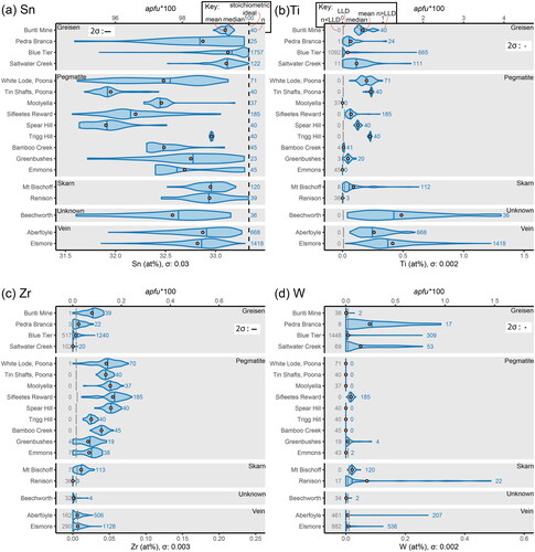
Figure 3. Intracrystalline and intercrystalline variability of substitutional elements in the cassiterite crystals analysed in this study, presented as violin plots in at% (bottom x-axis) and apfu*100 (top x-axis). Continued from Figure 2. (a) Variability in Fe. (b) Variability in Nb. (c) Variability in Mn. (d) Variability in Ta.

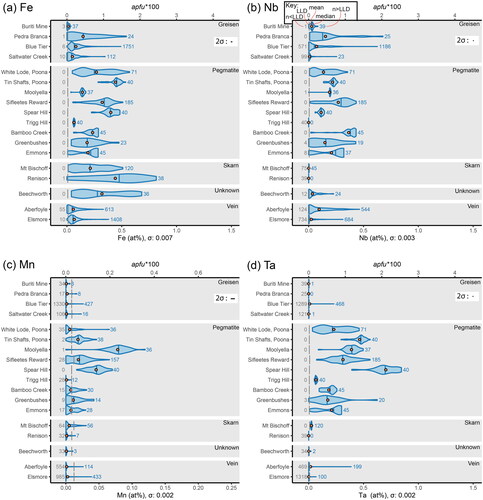
Figure 4. Oxygen fugacity buffer curves for the standard set (QIF to MH, left) with the reactions of interest to this study (right). The grey area represents the expected f_O2 of most cassiterite mineral systems (Bhalla et al., 2005; Ishihara, 1979; Linnen et al., 1995) and an expected upper T range of primary Sn-mineralising fluids in these systems (Heinrich, 1990).

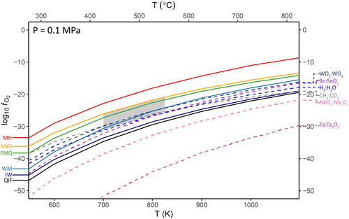
Figure 5. Oxygen fugacity speciation curves for oxidation states of interest, calculated at 800 K. The overall geometry of these curves is similar at lower temperatures. The grey area shows the projected range in f_O2 from Figure 4. The mid-points (equal activities) of the QIF, WM, QFM and MH buffers are shown as dashed vertical lines, using the same colour scheme as Figure 4. (a) The magenta line displays the total proportion of Sn⁴⁺ as a function of f_O2 for the Sn:SnO₂ reaction, the black to grey lines display the total proportion of Fe species. (b) The dark pink line displays the total proportion of Ta⁵⁺ for the Ta:Ta₂O₅ equation, the light pink line the proportion of Nb⁵⁺ for the NbO₂:Nb₂O₅ equation. The blue line is the total proportion of W⁶⁺ for the WO₂:WO₃ equation, and black line is the total proportion of Ti⁴⁺ over the proportion of Ti³⁺. (c) The black to grey lines display the changing speciation of Mn species.

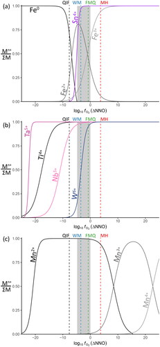
Figure 6. Lattice strain model for the possible substitution mechanisms of minor elements in cassiterite. (a) Predicted partition coefficients for ions only, including strain due to charge mismatch. (b) Partition coefficients using stoichiometrically averaged ionic radii (i.e. the ionic radius for the substitution of 2Nb⁵⁺Fe²⁺ is modelled as [2r_Nb5++r_Fe2+]/3). Charge is balanced in this instance, so strain only results from the combined radii mismatch. Note that the combination of larger and smaller cations results in an overall effective ionic radius similar to Sn⁴⁺.

Table 5. Possible substitution mechanisms for minor element incorporation into cassiterite. The different mechanisms are grouped into classes defined by the highest valency in the substitution reaction. The stoichiometric coupling reflects the ratio between cations in coupled substitutional pairs. The equations show the full substitution replacement reactions with Sn⁴⁺ into the cassiterite lattice. Each reaction has an assigned number, which will be used throughout the text. The ionic radius in six-fold (octahedral) coordination (Shannon & Prewitt, 1969) is shown for each cation (in Angstroms, Å), along with the radius for Sn⁴⁺ for comparison. Where the reaction contains multiple cations, the ionic radius shown is the stoichiometrically averaged radius for that reaction. An asterisk (*) denotes substitution reactions disregarded or not considered in previous literature.

Class, Coupling
	Equation (Eq. #)	IR^(VI) (Å)
Trivalent, Uncoupled
Fe^3+ + 1/3 Fei^3+ ⇌ Sn^4+ + □i	(1)	0.645
Fe^3+ + OH^– ⇌ Sn^4+ + O^2–	(2)	0.645
Tetravalent, Uncoupled
Si^4+ ⇌ Sn^4+	(3)	0.400
Mn^4+⇌ Sn^4+	(4)*	0.530
Ti^4+⇌ Sn^4+	(5)	0.605
W^4+⇌ Sn^4+	(6)	0.660
Nb^4+⇌ Sn^4+	(7)	0.680
Ta^4+⇌ Sn^4+	(8)	0.680
Sn^4+		0.690
Zr^4+⇌ Sn^4+	(9)	0.720
Pentavalent, 1:1
Nb^5+ + Fe^3+ ⇌ 2Sn^4+	(10)	0.643
Ta^5+ + Fe^3+ ⇌ 2Sn^4+	(11)	0.643
Nb^5+ + Mn^3+ ⇌ 2Sn^4+	(12)	0.643
Ta^5+ + Mn^3+ ⇌ 2Sn^4+	(13)	0.643
Pentavalent, 2:1
2Nb^5+ + Fe^2+ ⇌ 3Sn^4+	(14)	0.687
2Ta^5+ + Mn^2+ ⇌ 3Sn^4+	(15)	0.687
2Nb^5+ + Fe^2+ ⇌ 3Sn^4+	(16)	0.703
2Ta^5+ + Mn^2+ ⇌ 3Sn^4+	(17)	0.703
2W^5+ + Fe^2+ ⇌ 3Sn^4+	(18)*	0.673
2W^5+ + Mn^2+ ⇌ 3Sn^4+	(19)*	0.690
Hexavalent, 1:1
W^6+ + Fe^2+ ⇌ 2Sn^4+	(20)	0.690
W^6+ + Mn^2+ ⇌ 2Sn^4+	(21)*	0.635
Hexavalent, 1:2
W^6+ + 2Fe^3+ ⇌ 3Sn^4+	(22)	0.630
W^6+ + 2Mn^3+ ⇌ 3Sn^4+	(23)*	0.587

Table 6. Existing evidence for the substitution mechanisms outlined in Table 5. Each cell contains a tick (✓) if the evidence is in favour of the substitution mechanism, a cross (×) if the evidence does not support this mechanism, and a question mark (?) if the evidence is ambiguous or uncertain. The analytical methods are also described in each cell, as one of stoichiometric analysis via electron probe microanalysis (EPMA), direct measurement of oxidation states via electron paramagnetic resonance (EPR) or Mössbauer Spectroscopy (Möss), or consideration of the local electronic environment via cathodoluminescence theory (CL). Direct measurement of OH content by Fourier Transform Infrared spectroscopy (FTIR) is also included.

	Reference	a	b	c	d	e	f	g	h	i	j	k	l
(Eq.#)	Equation
(1)	Fe^3+ + 1/3 Fei^3+		✓EPR					×EPMA			×EPMA	×EPMA
(2)	Fe^3+ + OH^-			✓EPR	✓Möss	✓EPR	? EPMA	×EPMA	✓FTIR	✓FTIR	×EPMA	×EPMA	? EPMA
(3)	Si^4+	✓CL
(5)	Ti^4+	✓CL	✓EPR			✓EPR	✓EPMA	✓EPMA			✓EPMA		✓EPMA
(6)	W^4+	? CL			? EPMA						×EPMA
(7)	Nb^4+				? EPMA						×EPMA
(8)	Ta^4+				? EPMA						×EPMA
(9)	Zr^4+							✓EPMA			✓EPMA
(10)	Nb^5+ + Fe^3+	? CL	✓EPR	✓EPR	× Möss	✓EPR	? EPMA	×EPMA			×EPMA	×EPMA	? EPMA
(11)	Ta^5+ + Fe^3+	? CL	✓EPR		× Möss		? EPMA	×EPMA			×EPMA	×EPMA	? EPMA
(12)	Nb^5+ + Mn^3+				× Möss		? EPMA	×EPMA			×EPMA	×EPMA	? EPMA
(13)	Ta^5+ + Mn^3+				× Möss		? EPMA	×EPMA			×EPMA	×EPMA	? EPMA
(14)	2Nb^5+ + Fe^2+	? CL			✓EPMA		✓EPMA	✓EPMA			✓EPMA	✓EPMA	✓EPMA
(15)	2Ta^5+ + Mn^2+	? CL			✓EPMA		✓EPMA	✓EPMA			✓EPMA	✓EPMA	✓EPMA
(16)	2Nb^5+ + Fe^2+				✓EPMA		✓EPMA	✓EPMA			✓EPMA	✓EPMA	✓EPMA
(17)	2Ta^5+ + Mn^2+				✓EPMA		✓EPMA	✓EPMA			✓EPMA	✓EPMA	✓EPMA
(20)	W^6+ + Fe^2+	? CL			×EPMA						? EPMA
(22)	W^6+ + 2Fe^3+	?CL			✓EPMA

a, Hall & Ribbe (1971); b, Izoret et al. (1985); c, Dusausoy et al. (1988); d, Möller et al. (1988); e, Ruck et al. (1989); f, Neiva (1996); g, Masau et al. (2000); h, Maldener et al., 2001; I, Losos & Beran (2004); j, Černý et al. (2004); k, Pal et al. (2007); l, Neiva (2008).

Table 7. Possible end-member phases for (limited) solid solution series with cassiterite, corresponding to the substitution mechanisms in Table 5 (listed under Eq.#). The class (Tet., Tetragonal; Orth., Orthorhombic; Mon., Monoclinic; Trig., Trigonal), symmetry (space group) and unit cell parameters (lengths in Å, angles in degrees) for each phase are also listed. Data sourced from mindat.org (accessed 5th April 2020), except where referenced. Phases synthesised in a laboratory, and not known in nature, are labelled as synthetic.

Phase	Formula	Eq. #	Class	Symmetry	a	b	c	β
Rutile group
Cassiterite^a	SnO2	–	Tet.	P42/mnm	4.7382(4)		3.1871(1)
Stishovite^a	SiO2	3	Tet.	P42/mnm	4.1790(4)		2.6649(4)
Pyrolusite^a	MnO2	4	Tet.	P42/mnm	4.3980(1)		2.8726(1)
Rutile^a,b	TiO2	5	Tet.	P42/mnm	4.5937(1)		2.9587(1)
Synthetic^c	NbO2	7	Tet.	P42/mnm	4.8464(1)		3.0316(1)
Synthetic^d	TaO2	8	Tet.	P42/mnm	4.709		3.065
Other M^4+O2
Quartz	SiO2	3	Trig.	P3121	4.9133		5.4053
α-Cristobalite	SiO2	3	Tet.	P41212	4.9709(1)		6.9278(2)
Anatase	TiO2	5	Tet.	I41/amd	3.7845		9.5143
Synthetic^e	WO2	6	Mon.	P21/c	5.650(5)	4.892(5)	5.550(5)	120.42(7)
Baddeleyite^f	ZrO2	9	Mon.	P21/b	5.1505	5.2116	5.3173	99.23
Zircon	ZrSiO4	3,9	Tet.	I41/amd	6.607(1)		5.982(1)
Columbite group^g
Tapiolite	Fe^2+Ta2O6	15	Tet.	P42/mnm	4.762		9.272
Tantalite-(Fe)	Fe^2+Ta2O6	15	Orth.	Pbcn	5.73	14.24	5.08
Tantalite-(Mn)	Mn^2+Ta2O6	17	Orth.	Pbcn	5.7661(8)	14.44	5.093
Columbite-(Fe)	Fe^2+Nb2O6	14	Orth.	Pbcn	5.7321(4)	14.266(1)	5.0503(4)
Columbite-(Mn)	Mn^2+Nb2O6	16	Orth.	Pbcn	5.7637(7)	14.433(2)	5.0832(8)
Excess M^3+
Hematite	Fe2O3	1	Trig.	R-3c	5.038(2)		13.772(12)
Goethite	α-FeO(OH)	2	Orth.	Pnma	4.608	9.956	3.0215
Varlamoffite^h	(Sn,Fe)(O,OH)2	2	– Not formally described –
Wolframite group
Ferberite	Fe^2+WO4	20	Mon.	P2/b	4.72	5.7	4.96	90
Hübnerite	Mn^2+WO4	21	Mon.	P2/b	4.8238(7)	5.7504(10)	4.9901(8)	91.18(1)

^aBolzan et al., 1997, references therein. ^bNaidu & Virkar, 1998 report up to 7 ± 4 mol% TiO₂ in synthetic SnO₂. ^cDisplays the dirutile structure, but with tetragonal symmetry (Rogers et al., 1969). ^dSchönberg et al., 1954 report probable continuous solid solution between TaO₂ and TiO₂, but limited solid solution with VO₂ (which has a modulated dirutile structure). ^eMagnéli et al., 1952. Structurally very similar to rutile (dirutile structure), the WO₆ octahedra are slightly more deformed and drawn together into doublets due to metal-metal bonds (Magnéli et al., 1955). ^fDhage et al., 2006 report up to 25 mol% ZrO₂ in synthetic SnO₂. ^gThe columbite group minerals display solid solution and a variable degree of cation order, resulting in a wide range of unit cell parameters (Ercit et al., 1995). A miscibility gap exists between the tapiolite structure and that of columbite-tantalite (Černý et al., 1992). ^hAn International Mineralogical Association (IMA) approved but ‘questionable’ species, yet to be formally described due to the lack of sufficiently sized crystals for proper analysis (Jambor et al., 1995; Sharko, 1971).

Figure 7. Binary plot of the substitutional relationship between Fe + Mn and W. The grey trend lines represent stoichiometries of 1:2 for Equations 22 and 23, 1:1 for Equations 20 and 21, and 2:1 for Equations 18 and 19. Points plotting in regions defined between these lines require a component of each bounding substitutional stoichiometry. Samples are grouped according to (a) pegmatitic and granite-hosted systems, (b) greisen systems, (c) vein-hosted systems, and (d) skarn systems. Note that the horizontal trend along the x-axis observed for Sifleetes Reward (in A) is due to the substitution of Fe coupled with Nb and Ta.

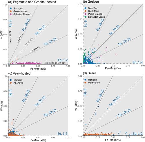
Figure 8. Monte Carlo simulation of a pure cassiterite EDS spectrum (black line), compared with simulated spectra of cassiterite doped with 1 apfu*100 of either Si (green line), Ta (red line) or W (blue line). The location of the Si Kα peak is indistinguishable from the combined X-ray emissions of the Ta Mα and Mβ lines. Overlap from the W Mαβ lines may also cause analytical difficulties in this region.

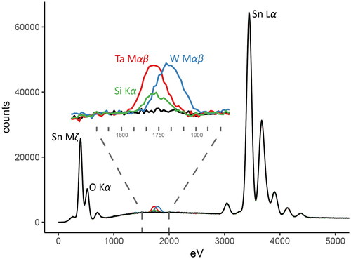
Figure 9. Net charge versus W for a cassiterite crystal from Saltwater Creek. The net charge is calculated as the sum of each component (in atomic percent) multiplied by their assumed charges (Nb⁵⁺, Ta⁵⁺, Sn⁴⁺, Ti⁴⁺, Zr⁴⁺, Fe²⁺, Mn²⁺), and assuming a stoichiometric concentration of 66.6̅ at% O. A linear correlation between charge and W concentration is observed. Charge is overbalanced (excess positive charge) if all W were assumed to be W⁶⁺, and underbalanced (excess negative charge) if all W were assumed to be W⁴⁺. Charge is only balanced if 25% of total W is W⁴⁺.

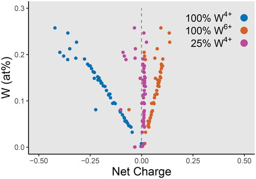
Figure 10. Binary plots of the substitutional relationships between Fe + Mn and Nb + Ta. The grey trend lines represent slopes of 1:1 for the stoichiometric substitutions of Equations 10–13 and 2:1 for Equations 14–17. Substitution via Equations 1 and 2 will plot along the x-axis, likewise, substitution via Equations 7 and 8 will plot along the y-axis. Points plotting in regions defined between these lines require a component of each bounding substitutional stoichiometry. Samples are grouped according to (a) pegmatitic and granite-hosted systems, (b) greisen systems, (c) vein-hosted systems, and (d) skarn systems.

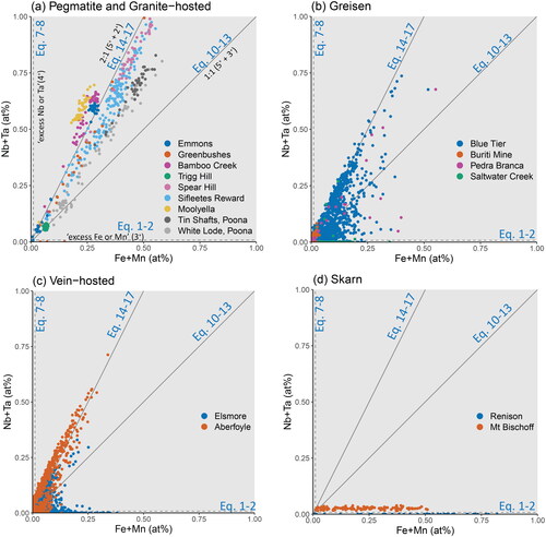
Figure 11. Projection of cassiterite samples onto the columbite–tantalite quadrilateral, showing Mn# vs Ta#. The tapiolite–tantalite miscibility gap of Černý et al. (1992) is included for reference, with the dotted field representing the range of compositions between coexisting pairs of tantalite and tapiolite, and the grey dashed lines representing the compositional bounds for single phases. (a) Cassiterite from silicate liquid systems. (b) Cassiterite from hybrid and aqueous fluid systems.

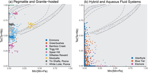
Figure 12. Ternary plots showing stoichiometric relationships between W, Fe + Mn, and Nb + Ta. These ternaries allow for comparison of W–Fe relationships in Nb + Ta bearing samples. The trend lines shown in Figure 10 project along the Fe + Mn and Nb + Ta join, and those shown in Figure 7 project along the Fe + Mn, and W join. Potential tie lines joining these substitutional stoichiometries are shown in grey. Transparency of the points decreases away from W concentrations at 2σ of the LLD, so that samples with the highest W contents are darker (more solid). Samples are grouped according to (a) pegmatitic and granite-hosted systems, (b) greisen systems, (c) vein-hosted systems, and (d) skarn systems.

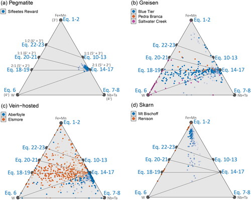
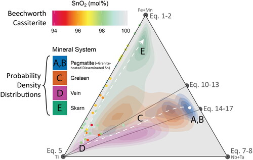
Figure 13. Ternary plots of the substitutional relationships between Ti, Fe + Mn, and Nb + Ta. The trend lines representing the 1:1 and 2:1 stoichiometric substitution reactions from Figure 10 project onto the Fe + Mn and Nb + Ta join, and tie lines joining these to the Ti apex are shown in grey. Colour represents the total SnO₂ content of each analysis, and the colour scheme was chosen to visually down-weight values close to stoichiometric SnO₂ (i.e. those with little to no substituting elements present). Samples are grouped according to (a) pegmatitic and granite-hosted systems, (b) greisen systems, (c) vein-hosted systems, and (d) skarn systems.

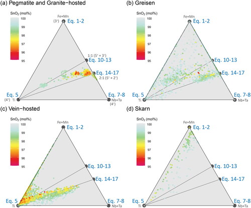
Figure 14. The Ti–(Fe + Mn)–(Nb + Ta) ternary diagram from Figure 13, with the data from each sub-figure (Figure 13a–d) contoured as probability density distributions, coloured according to (a, b) pegmatite and granite-hosted disseminated Sn systems, (c) greisen systems, (d) vein systems, and (e) skarn systems. Analyses from the cassiterite crystal from Beechworth, which has an unknown paragenesis, are plotted as points with the same colour scheme as Figure 13.

Bennett, J. M., Kemp, A. I. S., & Roberts, M. P. (2020). Microstructural controls on the chemical heterogeneity of cassiterite revealed by cathodoluminescence and elemental X-ray mapping. American Mineralogist, 105(1), 58–76. https://doi.org/10.2138/am-2020-6964

 Web of Science ®Google Scholar

Grundmann, G., & Morteani, G. (1998). Alexandrite, emerald, ruby, sapphire and topaz in a biotite–phlogopite fels from Poona, Cue District, Western Australia. Australian Gemmologist, 20, 159–167.

 Google Scholar

Jacobson, M. I., Calderwood, M. A., & Grguric, B. A. (2007). Guidebook to the pegmatites of Western Australia. Hesperian Press.

 Google Scholar

Marshall, D., Downes, P., Ellis, S., Greene, R., Loughrey, L., & Jones, P. (2016). Pressure-temperature-fluid constraints for the Poona Emerald Deposits, Western Australia: Fluid inclusion and stable isotope studies. Minerals, 6(4), 130. https://doi.org/10.3390/min6040130

 Web of Science ®Google Scholar

Sweetapple, M. T., & Collins, P. L. F. (2002). Genetic framework for the classification and distribution of Archean rare metal pegmatites in the North Pilbara Craton, Western Australia. Economic Geology, 97(4), 873–895. https://doi.org/10.2113/gsecongeo.97.4.873

 Web of Science ®Google Scholar

Partington, G. A., McNaughton, N. J., & Williams, I. S. (1995). A review of the geology, mineralization, and geochronology of the Greenbushes Pegmatite, Western Australia. Economic Geology, 90(3), 616–635. https://doi.org/10.2113/gsecongeo.90.3.616

 Web of Science ®Google Scholar

Ahmad, M. (1995). Genesis of tin and tantalum mineralization in pegmatites from the Bynoe area, Pine Creek Geosyncline, Northern Territory. Australian Journal of Earth Sciences, 42(5), 519–534. https://doi.org/10.1080/08120099508728222

 Web of Science ®Google Scholar

Summers, K. W. A. (1957). The mineral deposits of West Arm, Bynoe Harbour and Bamboo Creek Field, Northern Territory (BMR Record 1957/68). Bureau of Mineral Resources Geology and Geophysics.

 Google Scholar

Falster, A. U., Simmons, W. B., Webber, K. L., Dallaire, D. A., Nizamoff, J. W., & Sprague, R. A. (2019). The Emmons pegmatite, Greenwood, Oxford County, Maine. Rocks & Minerals, 94(6), 498–519. https://doi.org/10.1080/00357529.2019.1641021

 Google Scholar

Halley, S. W., & Walshe, J. L. (1995). A reexamination of the Mount Bischoff cassiterite sulfide skarn, western Tasmania. Economic Geology, 90(6), 1676–1693. https://doi.org/10.2113/gsecongeo.90.6.1676

 Web of Science ®Google Scholar

Walshe, J. L., Halley, S. W., Anderson, J. A., & Harrold, B. P. (1996). The interplay of groundwater and magmatic fluids in the formation of the cassiterite-sulfide deposits of western Tasmania. Ore Geology Reviews, 10(3-6), 367–387. https://doi.org/10.1016/0169-1368(95)00031-3

 Web of Science ®Google Scholar

Hutchinson, R. W. (1982). Geologic setting and genesis of cassiterite-sulfide mineralization at Renison Bell, Western Tasmania. Economic Geology, 77(1), 199–202. https://doi.org/10.2113/gsecongeo.77.1.199

 Google Scholar

Walshe, J. L., Solomon, M., Whitford, D. J., Sun, S.-S., & Foden, J. D. (2011). The role of the mantle in the genesis of tin deposits and tin provinces of eastern Australia. Economic Geology, 106(2), 297–305. https://doi.org/10.2113/econgeo.106.2.297

 Web of Science ®Google Scholar

Cochrane, G. W., & Bowen, K. G. (1971). Tin deposits of Victoria (pp. 1–72). Geological Survey of Victoria, Bulletin No. 60. Victorian Department of Mines.

 Google Scholar

Dunn, E. J., & Mahony, D. J. (1913). The Woolshed Valley, Beechworth (pp. 1–72). Geological Survey of Victoria, Bulletin No. 25. Victorian Department of Mines.

 Google Scholar

Blissett, A. H. (1959). The geology of the Rossarden-Storeys Creek District (Geological Survey of Tasmania, Bulletin No. 46). Tasmanian Department of Mines.

 Google Scholar

Brown, R. E., Stroud, W. J. (1993). Mineralisation related to the Gilgai Granite, Tingha-Inverell area. New England Orogen 1993 Conference Proceedings, 431–447.

 Google Scholar

Groves, D. I., Cocker, J. D., & Jennings, D. (1977). The Blue Tier Batholith. Geological Survey of Tasmania, Bulletin No. 55. Tasmania Department of Mines.

 Google Scholar

Reid, A. M., & Henderson, Q. J. (1928). Blue Tier Tin Field. Geological Survey of Tasmania, Bulletin No. 38. Tasmania Department of Mines. Hobart.

 Google Scholar

Keid, H. G. W. (1951). Memorandum—investigation lease no. 31M/50 Coles Bay [MRT document UR1951 070 73]. Mineral Resources Tasmania.

 Google Scholar

Twelvetrees, W. H. (1901). Report of the coalfield of Llandaff, the Denison and Douglas Rivers, on deposits of tin ore on Schouten Main, and on outcrops of quartz near Buckland (Tech. rep.). Tasmanian Government Geologist’s Office.

 Google Scholar

Botelho, N. F., & Moura, M. A. (1998). Granite-ore deposit relationships in Central Brazil. Journal of South American Earth Sciences, 11(5), 427–438. https://doi.org/10.1016/s0895-9811(98)00026-1

 Web of Science ®Google Scholar

Lenharo, S. L. R., Moura, M. A., & Botelho, N. F. (2002). Petrogenetic and mineralization processes in Paleo- to Mesoproterozoic rapakivi granites: Examples from Pitinga and Goiás, Brazil. Precambrian Research, 119(1-4), 277–299. https://doi.org/10.1016/s0301-9268(02)00126-2

 Web of Science ®Google Scholar

Bhalla, P., Holtz, F., Linnen, R. L., & Behrens, H. (2005). Solubility of cassiterite in evolved granitic melts: Effect of t, fO2, and additional volatiles. Lithos, 80(1-4), 387–400. https://doi.org/10.1016/j.lithos.2004.06.014

 Web of Science ®Google Scholar

Ishihara, S. (1979). Lateral variation of magnetic susceptibility of the Japanese granitoids. The Journal of the Geological Society of Japan, 85(8), 509–523. https://doi.org/10.5575/geosoc.85.509

 Google Scholar

Linnen, R. L., Pichavant, M., Holtz, F., & Burgess, S. (1995). The effect of fO2 on the solubility, diffusion, and speciation of tin in haplogranitic melt at 850 °C and 2 kbar. Geochimica et Cosmochimica Acta, 59(8), 1579–1588. https://doi.org/10.1016/0016-7037(95)00064-7

 Web of Science ®Google Scholar

Heinrich, C. A. (1990). The chemistry of hydrothermal tin(–tungsten) ore deposition. Economic Geology, 85(3), 457–481. https://doi.org/10.2113/gsecongeo.85.3.457

 Web of Science ®Google Scholar

Shannon, R. D., & Prewitt, C. T. (1969). Effective ionic radii in oxides and fluorides. Acta Crystallographica Section B Structural Crystallography and Crystal Chemistry, 25(5), 925–946. https://doi.org/10.1107/S0567740869003220

 Web of Science ®Google Scholar

Hall, M. R., & Ribbe, P. H. (1971). An electron microprobe study of luminescence centers in cassiterite. American Mineralogist, 56(1-2), 31–45.

 Web of Science ®Google Scholar

Izoret, L., Marnier, G., & Dusausoy, Y. (1985). Caracterisation cristallochimique de la cassiterite des gisements d’etain et de tungstene de Galice, Espagne. The Canadian Mineralogist, 23(2), 221–231.

 Google Scholar

Dusausoy, Y., Ruck, R., & Gaite, J. M. (1988). Study of the symmetry of Fe3+ sites in SnO2 by electron paramagnetic resonance. Physics and Chemistry of Minerals, 15(3), 300–303. https://doi.org/10.1007/BF00307520

 Web of Science ®Google Scholar

Möller, P., Dulski, P., Szacki, W., Malow, G., & Riedel, E. (1988). Substitution of tin in cassiterite by tantalum, niobium, tungsten, iron and manganese. Geochimica et Cosmochimica Acta, 52(6), 1497–1503. https://doi.org/10.1016/0016-7037(88)90220-7

 Web of Science ®Google Scholar

Ruck, R., Dusausoy, Y., Trung, C. N., Gaite, J.-M., & Murciego, A. (1989). Powder EPR study of natural cassiterites and synthetic SnO2 doped with Fe, Ti, Na and Nb. European Journal of Mineralogy, 1(3), 343–352. https://doi.org/10.1127/ejm/1/3/0343

 Web of Science ®Google Scholar

Neiva, A. M. R. (1996). Geochemistry of cassiterite and its inclusions and exsolution products from tin and tungsten deposits in Portugal. The Canadian Mineralogist, 34(4), 745–768.

 Google Scholar

Masau, M., Cerny, P., & Chapman, R. (2000). Exsolution of zirconian–hafnian wodginite from manganoan–tantalian cassiterite, Annie Claim #3 Granitic Pegmatite, Southeastern Manitoba, Canada. The Canadian Mineralogist, 38(3), 685–694. https://doi.org/10.2113/gscanmin.38.3.685

 Google Scholar

Maldener, J., Rauch, F., Gavranic, M., & Beran, A. (2001). OH absorption coefficients of rutile and cassiterite deduced from nuclear reaction analysis and FTIR spectroscopy. Mineralogy and Petrology, 71(1-2), 21–29. https://doi.org/10.1007/s007100170043

 Web of Science ®Google Scholar

Losos, Z., & Beran, A. (2004). OH defects in cassiterite. Mineralogy and Petrology, 81(3-4), 219–234. https://doi.org/10.1007/s00710-004-0040-x

 Web of Science ®Google Scholar

Černý, P., Chapman, R., Ferreira, K., & Smeds, S.-A. (2004). Geochemistry of oxide minerals of Nb, Ta, Sn, and Sb in the Varuträsk granitic pegmatite, Sweden: The case of an anomalous columbite–tantalite trend. American Mineralogist, 89(4), 505–518. https://doi.org/10.2138/am-2004-0405

 Web of Science ®Google Scholar

Pal, D. C., Mishra, B., & Bernhardt, H.-J. (2007). Mineralogy and geochemistry of pegmatite-hosted Sn-, Ta–Nb-, and Zr–Hf-bearing minerals from the southeastern part of the Bastar-Malkangiri pegmatite belt, Central India. Ore Geology Reviews, 30(1), 30–55. https://doi.org/10.1016/j.oregeorev.2005.10.004

 Web of Science ®Google Scholar

Neiva, A. M. R. (2008). Geochemistry of cassiterite and wolframite from tin and tungsten quartz veins in Portugal. Ore Geology Reviews, 33(3-4), 221–238. https://doi.org/10.1016/j.oregeorev.2006.05.013

 Web of Science ®Google Scholar

Černý, P., Ercit, T. S., & Wise, M. A. (1992). The tantalite–tapiolite gap; natural assemblages versus experimental data. The Canadian Mineralogist, 30(3), 587–596.

 Google Scholar