Assessing the consistency and reliability of the line intercept transect method in coral cover estimation using structure from motion photogrammetry techniques

Figures & data

Figure 1. Study area and surveyed reefs. NS01, NS02 and NS03 located on Fiery Cross Reef, NS04 and NS05 located on Thitu Island Reef. The red lines represent approximately the position of the transects.

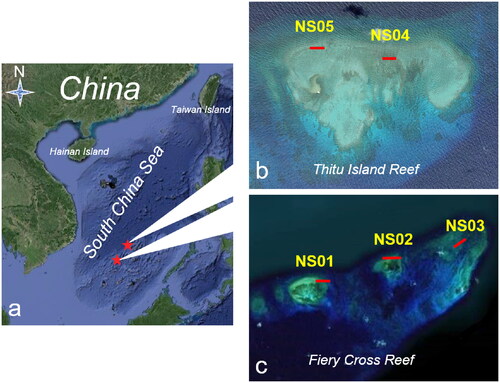
Figure 2. Workflow of methods used to derive the orthomosaics using SfM and subsequent analysis. (a) Laying a transect with the measuring tape and acquiring overlapping images and POS data. (b) Using the Agisoft Metashape to process the images and POS data and to generate orthomosaics of each transect. (c) Orthomosaics of five transects after buffering analysis within ArcGIS.

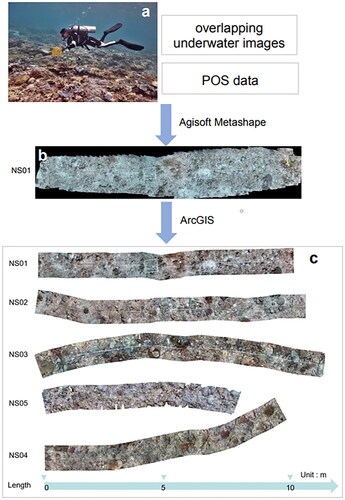
Table 1. Processing workflow and parameters in Metashape.

Processing workflow	Parameters
Add photos	–
Import reference	–
Align photos	Accuracy: High Generic preselection: Yes Reference preselection: Source
Build model	Surface type: Arbitrary Source data: Depth maps Interpolation: Enabled Quality: High Filtering mode: Disabled
Build texture	Texture: Diffuse map Source data: Images Mapping mode: Adaptive orthophoto Blending mode: Mosaic Enable hole filling: Yes Enable ghosting filter: Yes
Build orthomosaic	Projection type: Geographic (Local Coordinates (m)) Surface: Model Blending mode: Mosaic Refine seamlines: Yes Enable hole filling: Yes

Table 2. Some results on image acquisition and data processing.

Sites	NS01	NS02	NS03	NS04	NS05
The number of images	185	180	156	160	120
Pixel resolution/mm	0.24	0.15	0.29	0.27	0.36
average photography height/m	0.92	0.58	1.10	1.04	1.37
Width of the transect/m	1.0	1.0	1.0	1.0	1.0
length of the transect/m	10.90	10.22	11.56	9.72	8.02
‘Scale length’ of the transect/m	10.90	11.00	11.96	10.62	8.47

Figure 3. Statistics in data processing (NS01). (a) Camera locations are marked with a black dot, and image overlap is represented by different colors. (b) Camera locations and error estimates. Z error is represented by ellipse color. X, Y errors are represented by ellipse shape. Estimated camera location are marked with a black dot. (c) Two enlarged views of one reference scale segment.

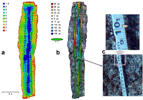
Figure 4. Statistical analysis of reference scale segments.

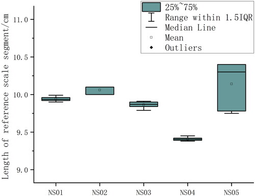
Figure 5. Analysis of coral cover from the orthomosaics. Green patches are coral colonies, red lines are the measuring tapes and blue lines are the virtual transects. The bottom three screenshots are coral recruits with different species and sizes.

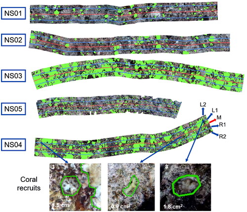
Figure 6. The estimates of percent coral cover by three methods. (a) The axes are the estimates of the three methods, which can clearly show the ranking of the estimates of the five sites. (b) The axes are the estimates of the five sites, including only the results of LIT and LITO.

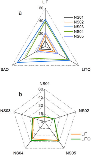
Table 3. Data quality and accuracy.

Sites		NS01	NS02	NS03	NS04	NS05
RMS reprojection error/pix		0.85	0.91	0.99	0.86	0.49
Reference scale segments	Range of values/cm	9.90–9.99	10.00–10.10	9.79–9.91	9.38–9.45	9.75–10.40
	Mean value/cm	9.94	10.06	9.86	9.41	10.14
	Sample standard deviation	0.0320	0.0516	0.0401	0.0207	0.2964
Scaling factor		0.994	1.006	0.986	0.941	1.014

Figure 7. Comparative analysis of the LITO and SAO methods. (a) The blue pellets represent each coral colony extracted. To highlight the distribution of coral colonies’ size at each site, the data were transformed using the log₂. (b) A larger view of the orange section of Figure 7(a) makes the distribution of coral recruits clearer. (c) The abundance of corals involved in the estimate of coral cover by the LITO and SAO methods and proportions of coral recruits.

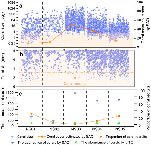
Figure 8. Estimates of percent coral cover by LITO and SAO.

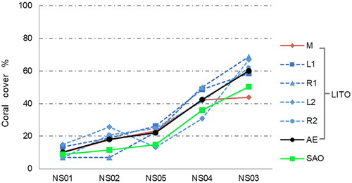
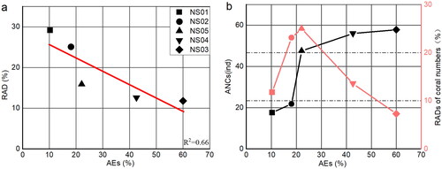
Figure 9. (a) The relationship between AEs and RADs of coral cover estimates by LITO. (b) The relationship between AEs and ANCs and RADs of coral abundances.