Figures & data
Figure 1. (a) Chemical structures of human metabolites of benzene. Source: Rappaport et al. (Citation2010). (b) Pathway schematic showing major metabolites (blue) and metabolizing enzymes (black) [muconic acid (MA) not shown]. Right side: side pathway schematic is from: https://www.wikipathways.org/index.php/Pathway:WP3891#nogo2.
![Figure 1. (a) Chemical structures of human metabolites of benzene. Source: Rappaport et al. (Citation2010). (b) Pathway schematic showing major metabolites (blue) and metabolizing enzymes (black) [muconic acid (MA) not shown]. Right side: side pathway schematic is from: https://www.wikipathways.org/index.php/Pathway:WP3891#nogo2.](/cms/asset/89b5f56e-d68e-47f9-8a80-d7ba6254999a/itxc_a_1860903_f0001_c.jpg)
Figure 2. Compartmental structure of a recent PBPK model for human metabolism of benzene. (Source: Knutsen et al. Citation2013).
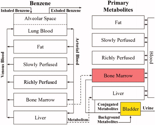
Figure 3. Comparison of benzene PBPK model predictions (solid lines) and uncertainty bands (dashed lines, representing ±2 standard deviations) to data (points) not used in building the model. MA: muconic acid; PMA: phenylmercapturic acid; PH: phenol; CAT: catechol; HQ: hydroquinone; BT: benzenetriol. (Source: Knutsen et al. Citation2013).
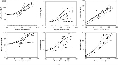
Figure 4. Proposed Bayesian network (BN) model structure. (Source: Hack et al. Citation2010). 8-OHdG: 8-hydroxyguanosine (a biomarker of oxidative stress); CFU-GEMM: colony-forming unit-granulocyte, erythrocyte, monocyte, megakaryocyte (a precursor to RBCs and WBCs); BFU-E: burst-forming unit-erythroid (a RBC precursor cell type); CFU-GM: colony forming unit – granulocyte-macrophage (a WBC precursor); RBC: red blood cell count; ttMA: trans, trans muconic acid; WBC: white blood cell count.
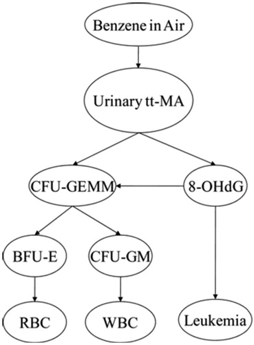
Figure 5. Uriinary metabolite levels vs. air benzene (AB) at AB concentrations below 3 ppm. (Metabolites are scaled so that 1 = mean value of each metabolite in the worker population.) Curves are non-parametric (smoothing) regression curves. Data points are for urinary benzene (UB). UB: urinary benzene; MA: E, E muconic acid; SPMA: S-phenylmercapturic acid; PH: urinary phenol; CA: urinary catechol; HQ: urinary hydroquinone. Data are from Price et al. (Citation2012).
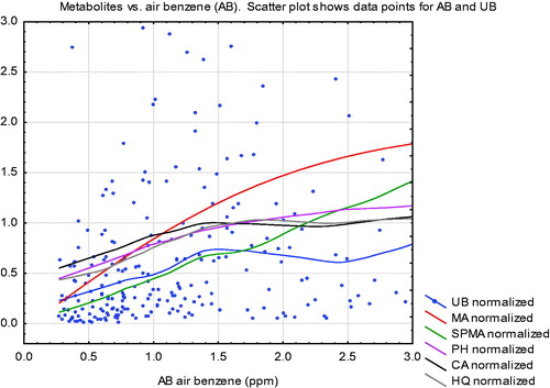
Figure 6. Frequency histograms (main diagonal), scatter plots with kernel smoothing regression curves (below diagonal) and linear (Pearson’s product moment) correlations and significance asterisks (above diagonal) (*0.05, **0.01, ***0.001). AT: air toluene; UT: urinary toluene; Creat: creatinine.
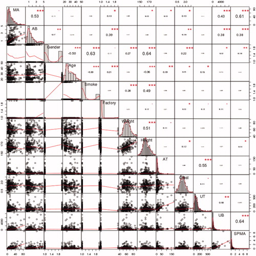
Figure 7. Visualizations of correlations. Upper left: Linear (Pearson’s) correlation corrgram (in color version, blue = positive correlation, red = negative, stronger correlations are darker). Upper right: Partial linear correlation corrgram. Lower left: Network visualization of linear correlations. In color version, green arcs represent positive correlations, red = negative, and thicker arcs and closer distances indicate stronger correlations. Lower right: Network visualization with polychloric correlations for binary variables.
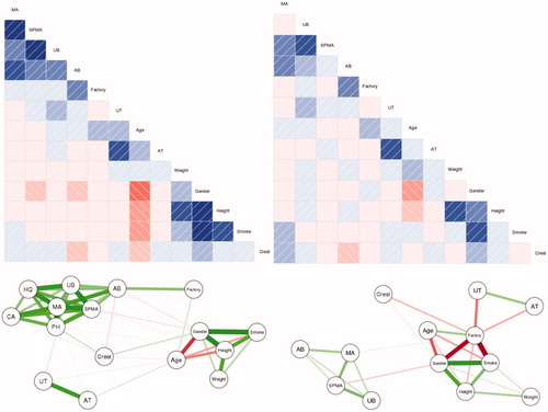
Figure 8. Partial dependence plots (PDPs) for urinary metabolites vs. air benzene (AB) concentration (ppm), controlling for Gender, Age, Smoke, Factory, Weight, Height, AT, Creatinine. PDPs were generated by the CAT software (http://cox-associates.com:8899/), which uses the randomForest package in R. (https://cran.r-project.org/web/packages/randomForest/randomForest.pdf).
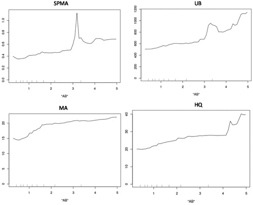
Figure 9. Air benzene contours show that air benzene can be predicted better from MA and UB (right side) than from MA and SPMA (left side).
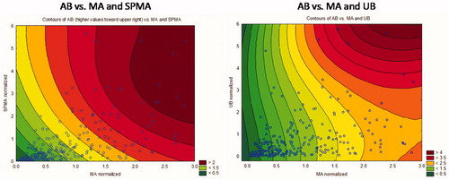
Figure 10. A Bayesian Network (BN) model learned from the Tianjin data. Arrows connect pairs of variables that are identified as being informative about (i.e. help to predict) each other.
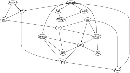
Figure 11. Individual Conditional Expectation (ICE) Plots for Production of Urinary Metabolites from Low Levels of Air Benzene Exposure (AB). Fraction of worker population in each cluster is given by “Prop.” (proportion) key in the upper left of each diagram. Vertical axes are scaled to show deviations from the overall population mean value. (Plots were generated by the CAT software using the ICEbox package in R (Goldstein et al. Citation2015). Plots control for individual Gender, Age, Smoke, Factory, Weight, Height, and AT by conditioning on their values in random forest analysis.
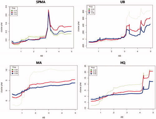
Figure 12. Categorized box-and-whisker plots show substantial interindividual variability in production of urinary metabolites (clockwise from upper left: normalized SPMA, UB, MA, HQ values, scaled so that population mean = 1 for each metabolite). Metabolite production is sub-linear at low doses (AB < 3 ppm) (i.e. successive increases in AB by 1 unit generate larger increases in metabolites).
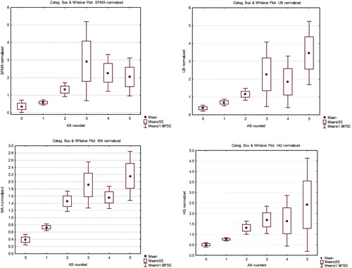
Figure 13. Joint scatter plots for SPMA and UB (left) and MA, UB, and SPMA (right) for workers exposed to 1 ppm (rounded to the nearest ppm) of benzene in air (AB = 1).
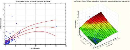
Figure 14. Women (upper curve) produce more SPMA than men at low concentrations (AB < 3 ppm) Vertical bars indicate approximate 95% confidence intervals.
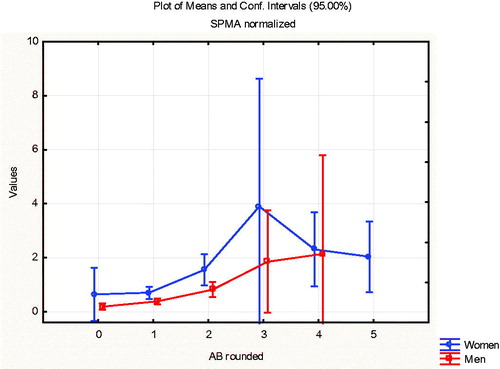
Figure 15. Urinary metabolites vs. AB (ppm) for 2 Individual Workers, each with 4 Repeated Measurements. (Top row SPMA; middle row UB; bottom row MA).
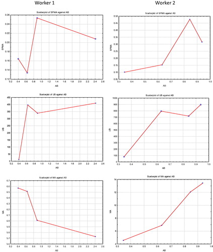
Figure 16. Top: Sub-linear production of benzene metabolites (UB on left; SPMA on right) by workers (partitioned into three clusters to indicate inter-individual heterogeneity), given AB. Bottom: Prediction of SPMA from UB. (Plots control for individual Gender, Age, Smoke, Factory, Weight, Height, and AT by conditioning on their values in random forest analysis.).
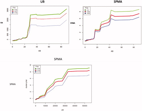
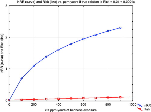
Figure 17. Comparison of linear and supralinear (spline) curves for lnRR vs. ppm-years of exposure, from Vlaanderen et al. (Citation2010).
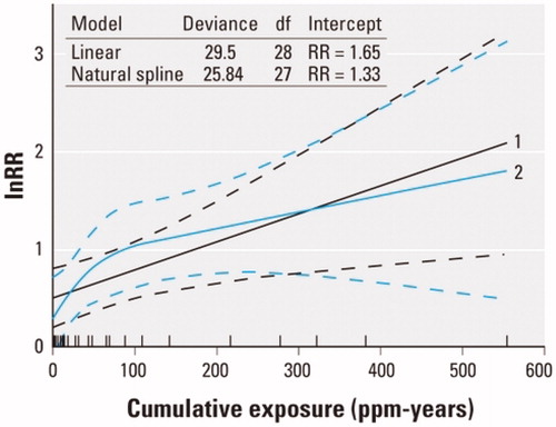
Figure 18. “Supralinearity” for lnRR is compatible with a linear exposure–response function.