
Figures & data
Figure 1. Schematic display of the solute density, , inside the sample during hydrogen charging (a) and subsequent modulation (b). (a) Applying a constant electrode potential
for a sufficient time interval leads to a homogeneous hydrogen concentration
inside the sample. Before equilibrium is reached, the difference
results in a current density
, Equation (Equation10
(10)
(10) ), of solutes through the surface, where
is the time-dependent density underneath the surface. (b) After reaching equilibrium, the electrode potential
, Equation (Equation2
(2)
(2) ), is modulated with respect to
giving rise to an oscillating variation of the solute density imposed by the surface,
, Equation (Equation11
(11)
(11) ). As a result of the modulation, a time-dependent density profile,
, inside the sample evolves, which is determined by the reaction- and diffusion-limitation of the process, Section 2.3. The difference between
and
leads again to a current density
of particles through the surface (Equation (Equation12
(12)
(12) ) and boundary condition according to Equation (Equation14
(14)
(14) )). (c) In comparison to (b) the situation for the entirely diffusion-limited case (boundary condition according to Equation (Equation16
(16)
(16) )). Note that figure parts b and c pertain to the special case of the diffusion–reaction model with the initial condition, Equation (Equation18
(18)
(18) ),
.
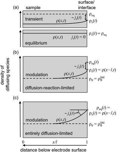
Figure 2. Amplitude (related to ) and phase angle
of the modulating part of the relative fraction
of loaded species in dependence of frequency-parameter
(plate: Equation (Equation30
(30)
(30) ); cylinder: Equation (Equation42
(42)
(42) )) for parameter (a) L = 1 and (b)
(plate: Equation (Equation25
(25)
(25) ); cylinder: Equation (Equation40
(40)
(40) )). Amplitude of plate: black dash-dotted line, Equation (Equation28
(28)
(28) ); amplitude of cylinder: black dotted line, Equation (Equation41
(41)
(41) );
for plate: red dashed line, Equation (Equation32
(32)
(32) );
for cylinder: red solid line, Equation (Equation45
(45)
(45) ); limiting case (b): Equations (Equation48
(48)
(48) ), (Equation49
(49)
(49) ), (Equation50
(50)
(50) ), and (Equation51
(51)
(51) ). Parameters:
m
/s;
m;
m/s (a),
(b).
![Figure 2. Amplitude (related to ρˆ/ρ0) and phase angle ϕ0 of the modulating part of the relative fraction n(t) of loaded species in dependence of frequency-parameter M∝ω (plate: Equation (Equation30(30) M=2l2ωD,(30) ); cylinder: Equation (Equation42(42) M=2r02ωD,(42) )) for parameter (a) L = 1 and (b) L→∞ (plate: Equation (Equation25(25) L=κlD,(25) ); cylinder: Equation (Equation40(40) L=κr0D(40) )). Amplitude of plate: black dash-dotted line, Equation (Equation28(28) n(t)=1−∑n=1∞2L2β¯n2(β¯n2+L2+L)[ρ0−ρ0iniρ0−12ρˆρ0M2β¯n2β¯n4+14M4]exp(−Dβ¯n2l2t)+2ρˆρ0LMCA2+B2sin(ωt+ϕ0)(28) ); amplitude of cylinder: black dotted line, Equation (Equation41(41) n(t)=1−∑n=1∞4L2β¯n2(β¯n2+L2)[ρ0−ρ0iniρ0−12ρˆρ0M2β¯n2β¯n4+14M4]exp(−Dβ¯n2r02t)+2ρˆρ0LM{2((J1Re)2+(J1Im)2)}1/2×{12M2((J1Re)2+(J1Im)2)+L2((J0Re)2+(J0Im)2)+ML[J1Im(J0Re−J0Im)−J1Re(J0Re+J0Im)]12}−1/2×sin(ωt+ϕ0)(41) ); ϕ0 for plate: red dashed line, Equation (Equation32(32) ϕ0=arctanAB+0 or π(32) ); ϕ0 for cylinder: red solid line, Equation (Equation45(45) ϕ0=arctanL[−J1Im(J0Re−J0Im)+J1Re(J0Re+J0Im)]−M((J1Re)2+(J1Im)2)L[J1Re(J0Re−J0Im)+J1Im(J0Re+J0Im)]+0 or π(45) ); limiting case (b): Equations (Equation48(48) ϕ0=arctansinM−sinhMsinM+sinhM(48) ), (Equation49(49) ϕ0=arctan−J1Im(J0Re−J0Im)+J1Re(J0Re+J0Im)J1Re(J0Re−J0Im)+J1Im(J0Re+J0Im).(49) ), (Equation50(50) nˆ=2ρˆρ01McoshM−cosMsin2M+sinh2M(50) ), and (Equation51(51) nˆ=2ρˆρ01M2((J1Re)2+(J1Im)2)((J0Re)2+(J0Im)2).(51) ). Parameters: D=3×10⁻¹¹ m2/s; l=r0=10−3 m; κ=3×10⁻⁸ m/s (a), →∞ (b).](/cms/asset/11680607-7eb6-4d9e-b85a-207391a62662/tphm_a_2333792_f0002_oc.jpg)
Figure 3. Density of loaded species , Equation (Equation34
(34)
(34) ), with respect to
in dependence of x (normalised to the half thickness l of the plate) for various values
(see legend in part (a1)). Surface located at
. Initial condition
, i.e. homogeneous density inside the plate in equilibrium with surface. Modulation amplitude
. Parameters:
m
/s;
m;
m/s (for
) or
m/s (for
). (a1)
: M = 5 (
1/s, black colour) and M = 20 (
1/s, red colour). (a2) Without transient part, i.e.
, Equation (Equation35
(35)
(35) ), exclusively; same parameters as for (a1). (b) M = 2 (
1/s):
(black colour) and L = 1 (red colour). (c) Periodic part
for
(black colour, with M = 10) and L = 1 (red colour, with M = 5). (Note legend in (c): solid line corresponds to
, unlike the other figure parts).
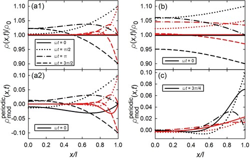
Figure 4. Real (Re) and negative imaginary part (−Im
) of complex impedance, Equation (Equation59
(59)
(59) ), of planar electrode in Nyquist-plot presentation for various values of L, Equation (Equation25
(25)
(25) ). The intersection with the real axis, i.e. −Im
, marks the limit
, whereas −Im
marks the limit
. For easy visualising, simple values in power of tens are used for the parameters, D (unit: m
/s), κ (unit: m/s), and l (unit: m). Variation of κ with D = 1 and l = 1: κ = 1 (L = 1, black solid), 10 (L = 10, blue dashed),
(
, blue dashed-dotted); variation of D with
and l = 1: D = 1 (L = 1, black solid), 10 (L = 0.1, black dashed),
(
, black dashed-dotted). Relations for the
-values at the frequency limits
and
are given in .
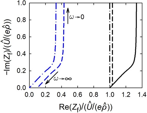
Table 1. Amplitude , real part of amplitude Re
and phase
of the complex impedance, Equation (Equation59
(59)
(59) ), and of the phase
, Equation (Equation32
(32)
(32) ), for
and
in the general case of diffusion and reaction limitation as well as in the special case of either reaction or diffusion limitation. Planar electrode; L, M according to Equations (Equation25
(25)
(25) ) and (Equation30
(30)
(30) ), respectively.