Hunting cooperation in a prey–predator model with maturation delay

Figures & data

Figure 1. Plots of two non-trivial nullclines $f_1(n,p)$ and $g_1(n,p)$ for $\sigma =0.5,\kappa =2,\alpha =1$ and $h_1$ varying from 0.1 to 0.6. As $h_1$ increases, the number of equilibrium point changes from 1 to 0.

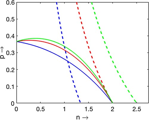
Figure 2. Plots of two non-trivial nullclines $f_1(n,p)$ and $g_1(n,p)$ for $\sigma =10,\kappa =1.2,\alpha =1$ and $h_1$ varying from 0.1 to 0.75. As $h_1$ increases, the number of equilibrium point changes from 1 to 0 ‘through 2’.

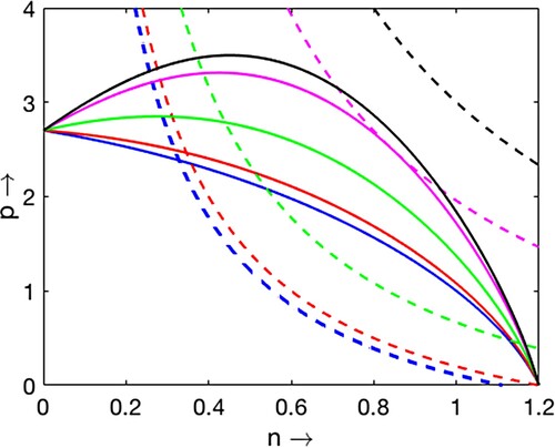
Figure 3. The bifurcation diagram with respect to the parameter $h_1$: (a) $\sigma =10,\kappa =1.2,\alpha =1$ and (b) $\sigma =10,\kappa =1.2,\alpha =2.217$.

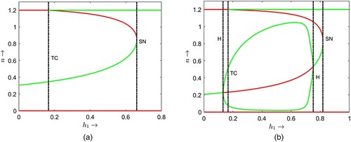
Figure 4. Plots of non-trivial prey nullcline $f_1(n,p)$ and predator nullcline $g_1(n,p,\tau )$ for $\sigma =10$, $\kappa =1.2$, $\alpha =1$, $h_1=0.1$, $\text{β}=0.1$ and three different values of τ: $\tau =0$, $\tau =1.5$, $\tau =3$.

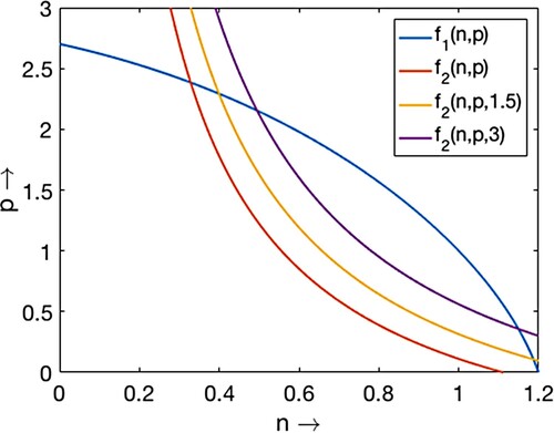
Figure 5. The bifurcation diagram with respect to the parameter $h_1$ with $\sigma =10$, $\kappa =1.2$, $\alpha =1$, $\text{β}=0.5$: (a) $\tau =0.3$ and (b) $\tau =0.6$.

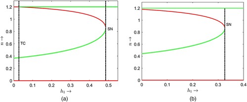
Figure 6. The bifurcation diagram with respect to the parameter $h_1$ with $\sigma =10$, $\kappa =1.2$, $\alpha =2.217$, $\text{β}=0.1$: (a) $\tau =0.05$ and (b) $\tau =0.06$.

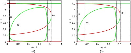
Figure 7. The bifurcation diagram with respect to the parameter $h_1$ with $\sigma =10$, $\kappa =1.2$, $\alpha =2.217$, $\text{β}=0.1$: (a) $\tau =0.0701$ and (b) $\tau =0.11$.

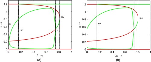
Figure 8. The bifurcation diagram with respect to the parameter $h_1$ with $\sigma =10$, $\kappa =1.2$, $\alpha =2.217$, $\tau =0.2$, $\text{β}=0.5$.

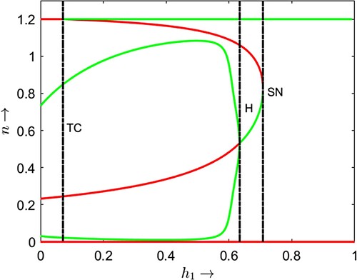
Figure 9. The bifurcation diagram with respect to the parameter τ with $\sigma =10$, $\kappa =1.2$, $\alpha =2$, $h_1=0.1$, $\text{β}=0.5$.

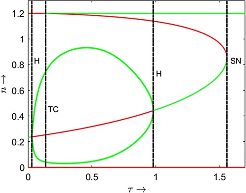
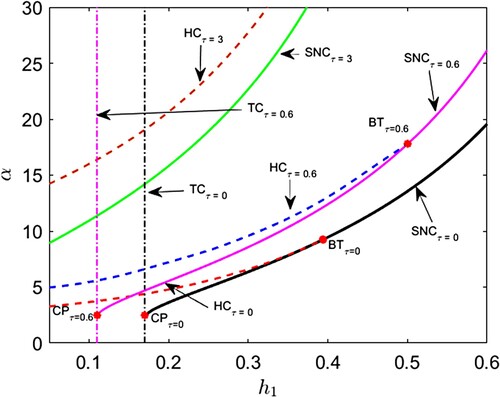
Figure 10. (Shift of bifurcation curves and bifurcation thresholds) $\sigma =0.4,\kappa =1.2,\text{ β}=0.1$. Black and magenta colour solid curves represent saddle node bifurcation curves (SNC) for $\tau =0$ and $\tau =0.6$ respectively. Red and blue colour broken curves represent Hopf bifurcation curves (HC) for $\tau =0$ and $\tau =0.6$ respectively. Black and magenta colour vertical dash–dot curves represent transcritical bifurcation curves for (TC) for $\tau =0$ and $\tau =0.6$ respectively. BT and CP stand for Bogdanov–Takens bifurcation threshold and cusp bifurcation thresholds respectively.

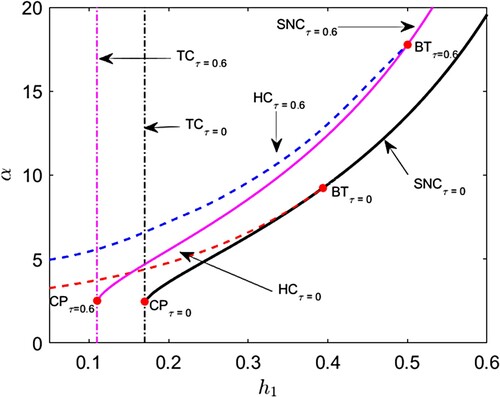
Figure 11. (Shift of bifurcation curves and bifurcation thresholds) $\sigma =0.4,\kappa =1.2,\text{ β}=0.1$. Black, magenta and green colour solid curves represent saddle node bifurcation curves (SNC) for $\tau =0$, $\tau =0.6$ and $\tau =3$ respectively. Red, blue and brown colour broken curves represent Hopf bifurcation curves (HC) for $\tau =0$, $\tau =0.6$ and $\tau =3$ respectively. Black and magenta colour vertical dash–dot curves represent transcritical bifurcation curves for (TC) for $\tau =0$ and $\tau =0.6$ respectively. BT and CP stand for Bogdanov–Takens bifurcation threshold and cusp bifurcation thresholds respectively.