The magnetic method as a tool to investigate the Werenskioldbreen environment (south-west Spitsbergen, Arctic Norway)

Figures & data

Figure 1. Lithostratigraphy of the Werenskioldbreen basin, modified after Stachnik et al. (2016). All subdivided units belong to the Heckla Hoek Succession.

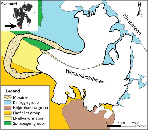
Table 1. Grouping of investigated samples into sets.

Set of samples	Sample
Nottinghambukta	NB1-11
North stream	WP100-119
South stream	WP1-11
Glacier river	WP12-18

Figure 2. Location map of analysed samples (based on Norwegian Polar Institute maps at http://toposvalbard.npolar.no/). The glacier front was drawn based on the Landsat 8 satellite image from 8 September 2015 (available from the US Geological Survey at https://earthexplorer.usgs.gov/).

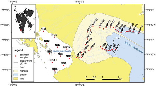
Figure 3. Distribution of χ_LF in the investigated area (based on Norwegian Polar Institute maps at http://toposvalbard.npolar.no/).

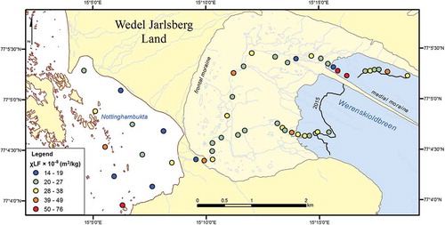
Figure 4. Distribution of χ_ARM in the investigated area (based on Norwegian Polar Institute maps at http://toposvalbard.npolar.no/).

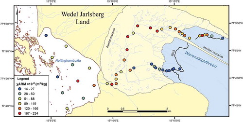
Figure 5. κ(T) conducted in the air with heating curves (red) and cooling curves (blue). (a, b) Typical diagrams for most samples of Nottinghambukta, characteristic also of the north stream and the glacier river. (c, d) Partial κ(T) analysis for the NB11 sample. (e, f) Typical diagrams for the south stream, characteristic also of the outside part of the bay. (g, h) Examples of untypical diagrams from the south stream. In the graphs in the right column (b, d, f, h) the heating curves are shown with enlarged scales on the y axes, providing more detail.

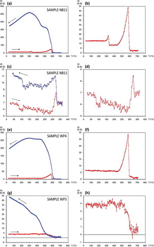
Figure 6. Example of hysteresis loops for a sample (a, b) with and (c, d) without pyrrhotite. The graphs on the right (b, d) display loops after paramagnetic correction.

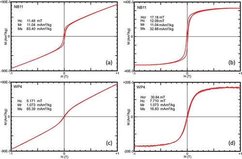
Figure 7. Day-Dunlop graph showing the hysteresis magnetization ratio (M_rs/M_s) versus coercivity ratio (H_cr/H_c) (Day et al. 1977; Dunlop 2002a, b). Dotted line represents theoretically calculated mixing curve of single-domain with superparamagnetic grains (SD + 10 nm SP). Dashed curves represent different mixing curves of single–domain and multi–domain particles (SD + MD).

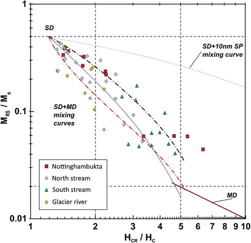
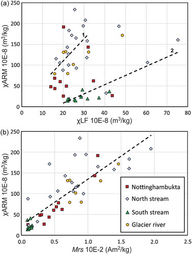
Figure 8. Plots of (a) χ_ARM versus χ_LF (King et al. 1982) and (b) anhysteretic magnetic susceptibility versus saturation magnetization (M_rs).

Stachnik Ł., Majchrowska E., Yde J.C., Nawrot A., Cichała–Kamrowska K., Ignatiuk D. & Piechota A. 2016. Chemical denudation and the role of sulfide oxidation at Werenskioldbreen, Svalbard. Journal of Hydrology 538, 177–193.

 Web of Science ®Google Scholar

Day R., Fuller M. & Schmidt V.A. 1977. Hysteresis properties of titanomagnetites: grain-size and compositional dependence. Physics of the Earth and Planetary Interiors 13, 260–267.

 Web of Science ®Google Scholar

Dunlop D.J. 2002a. Theory and application of the Day plot (Mrs/Ms versus Hcr/Hc) 1. Theoretical curves and tests using titanomagnetite data. Journal of Geophysical Research—Solid Earth 107, article no. 2056, doi: 10.1029/2001JB000486.

 Web of Science ®Google Scholar

King J.W., Banerjee S.K., Marvin J.A. & Özdemir Ö. 1982. A comparison of different magnetic methods for determining the relative grain size of magnetite in natural materials: some results from lake sediments. Earth and Planetary Science Letters 59, 404–419.

 Web of Science ®Google Scholar