The landscape in the gut microbiome of long-lived families reveals new insights on longevity and aging – relevant neural and immune function

Figures & data

Figure 1. Comparison of the gut microbiota between G3, G2 and G1 groups according to the 16S rRNA data. (a). Venn diagram of the observed ASVs in G3 (n = 11, aged 16 to 52 years [mean age, 37.1 years]), G2 (n = 30, aged 52 to 83 years [mean age, 71 years]) and G1 (n = 32, aged 100 to 108 years, [mean age, 101.7 years]) groups. (b-c). Alpha diversity indices of genera between three groups according to Estimate of richness (b), Shannon index (c). *p < .05; Wilcoxon rank-sum test. ns, not significant. (d). Principal coordinate analysis (PCoA) of the microbiota based on the Bray-Curtis distance between three groups. ANOSIM, R = 0.033, p = .175. (e). Bar plots showing the relative abundance of microbiota of three groups of individuals at phylum level, with different colors correspond to different phyla. (f). Bar plots showing the relative abundance of Firmicutes and Bacteroidetes in three groups. (g). Heat map showing the relative abundance of three groups of individuals at genus level. Only the significantly different genera between any two groups were displayed. Based on the different genera obtained by Wilcoxon rank sum test (Benjamini–Hochberg-corrected P value < .05), 10 samples were randomly returned from each group to form self-help samples. The average difference statistics of relative genus abundance were calculated and repeated 1000 times to determine whether the difference was significant according to 90% confidence interval. (h). Changes in the relative abundance of genera between G3, G2, and G1 subjects grouped according to the rejuvenation signature.

Figure 2. Bacterial correlation analysis based on relative abundance between G3, G2 and G1 groups. (a). Co-abundance groups interaction network. Node size represents the average abundance of each ASV. Lines between nodes represent correlations of each other, with the line width representing the correlation magnitude. The red ones represent positive correlations, and the blue ones represent negative correlations. Only lines whose absolute value of correlation coefficient greater than 0.70 were drawn, and unconnected nodes were omitted. (b). Group-level abundance differentiation of guilds. Data are visualized by boxplot. Box represents the interquartile range. The line inside the box represents the median. And whiskers denote the minimum and maximum value. *p < .05; **p < .01; Wilcoxon rank-sum test. ns, not significant. (c-e). Network plots describing co-occurrence of bacterial genera in the gut microbiota of G3, G2, and G1 group based on the Spearman correlation algorithms (r ≥ 0.7, FDR < 0.05). Bacterial genera with at least 0.1% of relative abundance in at least 20% of the samples in each group were plotted. Each node presents a bacterial genus. The node size indicates the relative abundance of each genus per group, and the density of the dashed line represents the Spearman coefficient. Red links stand for positive interactions between nodes, and green links stand for negative interactions. (f). Discrepancies of the genera co-occurrence networks between three groups based on the 16S rRNA data. Centralities (rank of the closeness) and discrepancies of nodes in G3, G2 and G1 co-occurrence networks were counted, respectively.

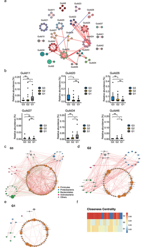
Figure 3. Comparison of the gut microbiota and gene functions between G3, G2, and G1 based on the metagenomic sequencing data. (a). Alpha diversity indices of species between three groups according to Shannon index. *p < .05; Wilcoxon rank-sum test. ns, not significant. (b). Heat map showing the relative abundance of individuals at different age stages at species level. Only the significantly differential genera were shown between any two groups in G3, G2, and G1 groups were displayed. Benjamini–Hochberg-corrected P value < .05; Wilcoxon rank-sum test. (c). Bar plot showing the relative abundance difference in MetaCyc pathways between three groups. Only the significantly differential pathways were shown between G3 and G1 individuals. (d). Bar plot showing the relative abundance difference in GBMs between three groups. Only the significantly different GBMs were shown between G3 and G1 individuals. (e). Genomic features of Odoribacter splanchnicus. The 3,788,833 bp genome containing 182 contigs, a N50 length of 30400 bp, a GC content of 43.5%. From the outer circle to the inner, it represents the length of contigs, coding sequences (CDS) on forward and reverse strands, tRNA, rRNA, tmRNA, CAZy annotation, GC content and GC skew curve, respectively. (f) Pie charts showing the function of Odoribacter splanchnicus genome at subcategory level based on RAST annotation. (g). The overview of ARGs in three groups. (h). Comparison of the number of ARGs between three groups. (i). Comparison of the number of ARG subtypes between three groups. (j-k). Abundance of significantly different ARG types between G3 and G1 individuals.

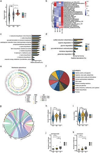
Figure 4. Odoribacter_splanchnicus correlations with other species at different age stages. (a-d). Correlations of Odoribacter splanchnicus with other species in 21–40, 41–60, 61–80 and 100–110 y old respectively. Spearman correlation algorithms (r ≥ 0.5,FDR<0.05). Red links stand for positive interactions between nodes, and green links stand for negative interactions.

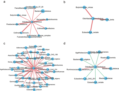
Figure 5. Classifiers for distinguishing G3 from G1 group and G2 from G1 group. (a). Receiver operating characteristic (ROC) curves for the G3 and G1 group were assessed by R Random Forest package. Only the top 20 significantly different genera between G3 and G1 individuals was used as predictors based on the 16S rRNA data. Another Chinese dataset as external validation set. Chinese young (n = 38) and centenarians (n = 48) from the SRA database under accession no. SRP107602. b. In order of importance, the genera used for predicting G3 and G1 groups were listed. (c). ROC curves for the G3 and G1 groups were assessed by R Random Forest package. Only the top 20 significantly different MetaCyc pathways between G3 and G1 individuals are used as predictors based on the metagenomic sequencing data. Sardinian dataset as external validation set. Sardinian young (n = 17) and centenarians (n = 19) from the European Nucleotide Archive (accession number PRJEB25514). (d). The MetaCyc pathways were ranked in order of importance for predicting G3 and G1 groups. (e). ROC curves for the G2 and G1 groups assessed by R Random Forest package. Using only the top 20 significantly different genera between G3 and G1 individuals as predictors based on the 16S rRNA data. Another Chinese dataset as external validation set. (f). Genera used to predict G2 and G1 groups were ranked in order of importance. (g). ROC curves for the G2 and G1 groups were assessed by R Random Forest package. Using only the top 20 significantly different MetaCyc pathways between G3 and G1 individuals as predictors based on the metagenomic sequencing data. Sardinian dataset as external validation set. (h). The MetaCyc pathways were ranked in order of importance for predicting G3 and G1 groups.

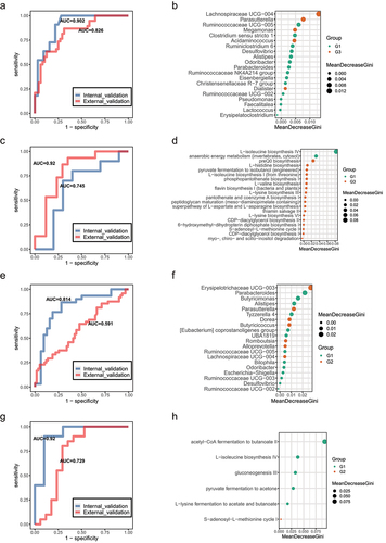
Figure 6. Associations between species, immune cytokines and pathways. (a-b). Analysis of the level of eight immune cytokines, Aβ, and BDNF in G3, G2 and G1 groups. Serum of all subjects was collected and detected by ELISA. The differences were calculated by t-test (*p < .05, **P < 0 .01, ***P < .005, ****P < .001). (c). Heatmap of associations between species and cytokines. (d). Heatmap of associations between MetaCyc pathways and cytokines. (e). Heatmap of associations between species and MetaCyc pathways. (f). Correlation between species, serum cytokines and MetaCyc pathways based on the Spearman correlation algorithms according to the metagenomic sequencing data (Benjamini–Hochberg-corrected P value < .05). Only the top 20 significantly different species and pathways between G2 and G1 individuals were used to calculate the correlation. In (c-e), only the top 20 significantly different species and MetaCyc pathways between G3 and G1 individuals were used to calculate correlation according to the metagenomic sequencing data. Spearman correlation, *p-value<0.05, **p-value<0.01.

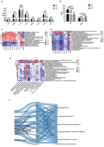
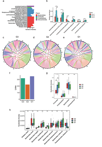
Figure 7. Inheritance at the species level in long-lived families. (a). Species that exist in at least half of long-lived families (n = 26) and show no significant differences in relative abundance between G3, G2 and G1 groups according to the 16S rRNA data. (b). Relative abundance of species presented in Figure 6a were shown in another Chinese dataset under accession no. SRP107602. Only the significantly differential species were shown between China_Y, China_E and China_C. **p < .01; *p < .05; Wilcoxon rank-sum test. ns, not significant. (c-e). A link was drawn for each strain shared between G3 individuals, G2 individuals and G1 individuals respectively according to the metagenomic sequencing data. (f). Enumeration of links drawn in Figure 6c-e. (g). Comparison of nucleotide diversity at the phylum level presented in Figure 2c. (h). Comparison of nucleotide diversity at the species level presented in Figure 6a. In (g-h), ***p < .001; **p < .01; *p < .05; Kruskal-Wallis with Dunn’s test. ns, not significant.

Data availability statement

All 16S rRNA and metagenomics raw data have been deposited into CNGB Sequence Archive (CNSA) of China National GeneBank DataBase (CNGBdb) with accession number CNP0002519.