Metaproteomics analysis of microbial diversity of human saliva and tongue dorsum in young healthy individuals

Figures & data

Figure 1. Laboratory workflow for saliva and tongue microbiome analysis (a). Tongue samples were collected with a sterile wooden spatula and transferred into sterile PBS. Salivation was stimulated by chewing a paraffin gum and the subjects spit into a Falcon tube®. Saliva was centrifuged and the resulting pellet was solved in TE-buffer and treated with ultrasonication. Proteins from saliva and tongue samples were precipitated with TCA and digested with trypsin. Peptide mixtures were measured with a Q Exactive™ Plus (LC-MS/MS). Bioinformatic workflow for metaproteomic data analysis (b). The Trans-Proteomic Pipeline was used for the following four steps: (1) Raw-data conversion to mzML-data format. (2) MS/MS database search by the Comet project for peptide identification based on a combined database (Human Swissprot + Human Oral Microbiome Database). (3) Validation of identified peptides. (4) Protein assignment and data filtering by stabilizing false discovery rates (mFDR, pepFDR) with a protFDR of 5.0 %. Finally, the online web-tool Prophane was applied to conduct taxonomic and functional prediction and the statistical analyses were performed in R.

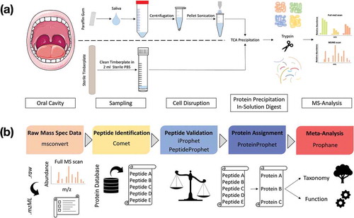
Figure 2. Venn diagrams displaying the number of identified metaproteins in the studied saliva and tongue samples for bacteria (a) and human species (c). Histograms of relative metaprotein abundances based on log₂ normalized spectral abundance factors (NSAF-values) [60] for bacterial (b) and human proteins (d). The figure emphasizes the distribution of metaproteins for saliva (blue), tongue (red) or shared between both (grey).

Figure 3. Heat trees of taxonomic composition of the healthy saliva (a) and tongue (b) microbiome. Coloration is defined by log₂ sum normalized spectral abundance factors (NSAF-values) [60]. The number of spectral counts for each branch determines its thickness.

Figure 4. Significant taxonomic profile differences on the genus level between saliva and tongue are displayed in the volcano plot (a) by depicting the results of a two-paired Wilcoxon signed rank test. The comparison plots (b) show the sum of the NSAF values for those genera identified as significantly higher abundant in saliva or on the tongue. Metaproteins in the group ‘heterogeneous’ could not be assigned unambiguously to a genus.

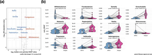
Figure 5. Illustration of taxonomic differences between saliva and tongue based on median over pairwise NSAF ratios (coloration) and the sum of spectral count (branch size). Genera marked with an * showed significant differences between both microbiomes according to a Wilcoxon signed rank test (Benjamini-Hochberg corrected p-value < 0.05).

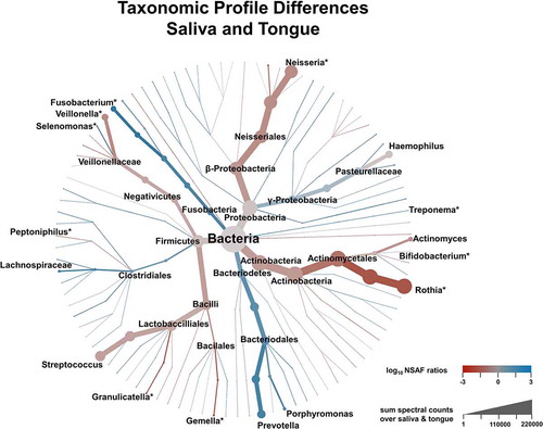
Figure 6. Comparison plots show the different relative abundances of bacterial metaprotein functions with significant differences, which were determined by a two-sided pairwise Wilcoxon signed rank test (p-value < 0.05) with a fold change of > 1.5. The calculated p-value has been corrected according to the Benjamini-Hochberg method.

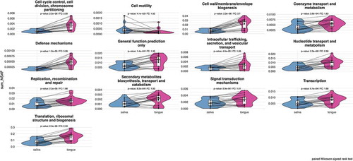
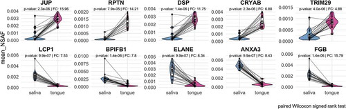
Figure 7. The coverage of the dynamic range of human proteins is shown by plotting the mean relative abundance for saliva and tongue (a). The human proteins are named according to their gene names and show for saliva and tongue a selection of proteins with highest and lowest abundances (grey). Data points in red and blue display proteins with a fold change > 1.5 and a p-value < 0.5 (paired Wilcoxon signed rank test) comparing saliva and tongue (a). Proteins with the largest changes are highlighted with their gene names (A/B).

Figure 8. Representation of the top five proteins with the highest increase or decrease regarding to their relative abundance in saliva or on the tongue based on paired Wilcoxon signed rank test (p-value < 0.05).

Zybailov B, Mosley AL, Sardiu ME, et al. Statistical analysis of membrane proteome expression changes in Saccharomyces cerevisiae. J Proteome Res. 2006;5:2339–2347.

 PubMed Web of Science ®Google Scholar