
Figures & data
Figure 1. Naringenin on the left and naringin on the right.
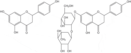
Figure 2. Nifedipine (dimethyl 2,6-dimethyl-4-(2-nitrophenyl)-1,4-dihydropyridine-3,5-dicarboxylate) and nisoldpine (3-isobutyl 5-methyl 2,6-dimethyl-4-(2-nitrophenyl)-1,4-dihydropyridine-3,5-dicarboxylate).
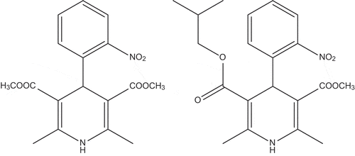
Figure 3. Bergamottin.
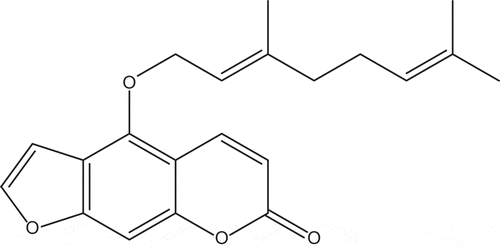
Figure 4. A graph of the surviving fraction against half-life for the simplified equation.
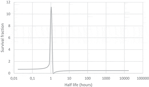
Table 1. The number of days lost from the life expectancy of a person requiring low to medium care evacuated from a care home in the Fukushima area.
Table 2. Examples of different accidents rated on the INES scale.
Table 3. Thermodynamic stability constants for acetate complexes of uranium and plutonium.
Figure 5. The coordination environment of the cesium in cesium uranyl acetate. The cesium is blue, the uranium atoms are yellow, the oxygens are red, the carbons are dark grey and the hydrogens are light grey.
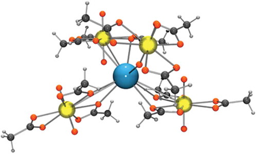
Figure 6. The coordination sphere of a potassium in potassium uranyl acetate. The potassium is purple, the uraniums are yellow, the oxygens are red, the carbons are dark grey and the hydrogens light grey.
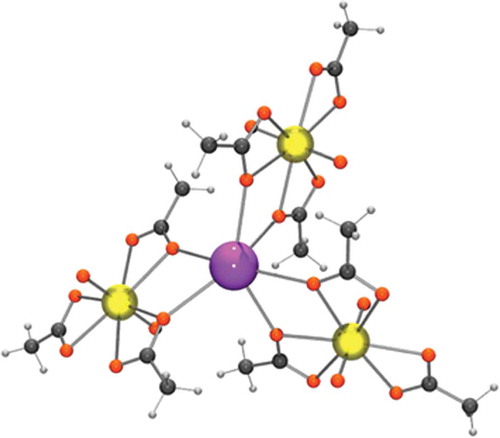
Table 4. Main radionucldies released in the Kyshtym accident.
Figure 7. A cobalt dicarbolide anion. The cobalt atom is blue, the boron atoms are gold colour, the carbon atoms are dark grey and the hydrogen atoms are light grey.
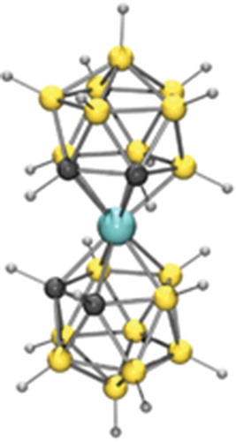
Figure 8. The structure of dipotassium copper ferrocyanide. Potassium atoms are pale blue, iron atoms are green, copper atoms are orange, carbon atoms are dark grey and nitrogen atoms are dark blue.
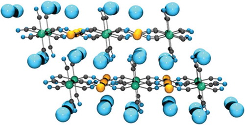
Figure 9. The structure of potassium nickel ferrocyanide.
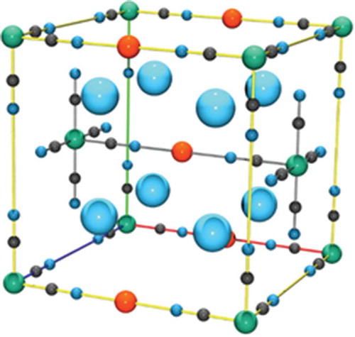
Figure 10. The anion in ammonium molydophosphate [Mo12O36·PO4]3−.
![Figure 10. The anion in ammonium molydophosphate [Mo12O36·PO4]3−.](/cms/asset/df2cc14c-f6a9-453c-9c45-495a7b9e9fec/oach_a_1450944_f0010_c.jpg)
Figure 11. Four views of an alpha uranium unit cell.
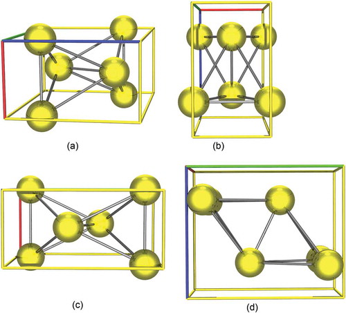
Table 5. Summary of rules for counting atoms in unit cells.
Figure 12. The layers in Fe2U.
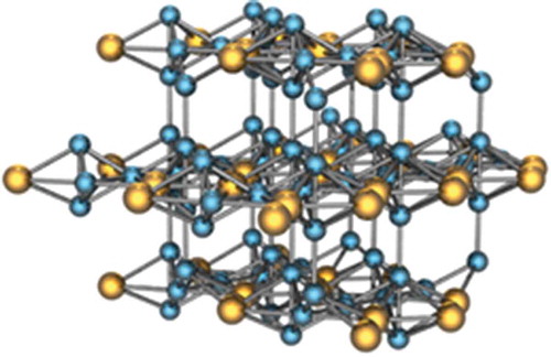
Figure 13. A unit cell of UNi2, the nickel atoms are in green while the uranium atoms are in yellow.
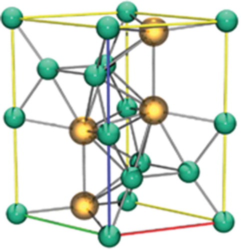
Figure 14. A unit cell of UNi5, the nickel atoms are in green while the uranium atoms are in yellow.
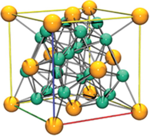
Figure 15. A unit cell of U11N16, the nickel atoms are in green while the uranium atoms are in yellow.
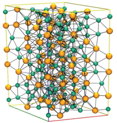
Figure 16. A unit cell of UNi4.
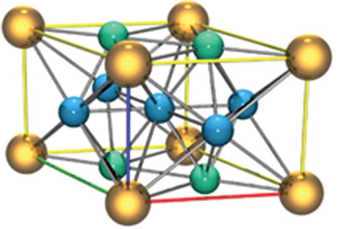
Table 6. Half-lives and fission yields of cesium, tellurium and iodine.
Table 7. Details of the layers on a stainless steel exposed to iodine.
Figure 17. A diagram of the layers on the surface of a stainless steel exposed to iodine.
Table 8. Groups of fission products in the prediction of the behaviour of magnox fuel during an accident.
Table 9. Two magnesium alloys, the amounts of elements are in % (w/w).
Figure 18. A diagram of the Chernobyl core and the control rods. H are the areas of the core with the highest K∞ due to the lowest burnup, M are areas with medium K∞ and L are the areas with the lowest K∞. The boron containing adsorbing sections are shown in black and the graphite displacers in grey.
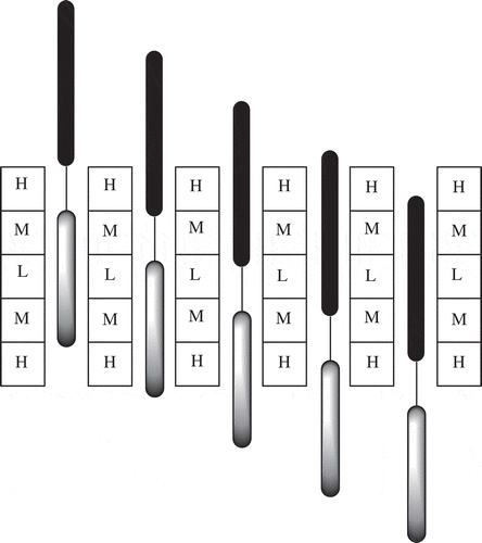
Table 10. Fission yields for nuclides with a mass of 131.
Table 11. Fission products with a mass of 103.
Table 12. Fission products with a mass of 99.
Table 13. Details of excel calculations used to test the dynamic range of the calculation process.
Figure 19. The error on the calculation as a function of Q.
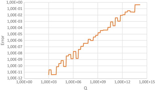
Table 14. ARF and RF values for plutonium compounds in fires.
Figure 20. On the left the original Marinelli beaker with a GM tube in the central cavity while on the right is the modern version with a solid state detector in the cavity at the bottom.
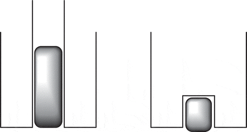
Figure 21. Gamma spectrum of 40K.
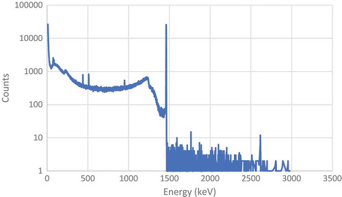
Table 15. Details of some noble gas radionuclides formed in a fission reactor.
Figure 22. Pie chart of the iodine activity ratio at the point of fission.
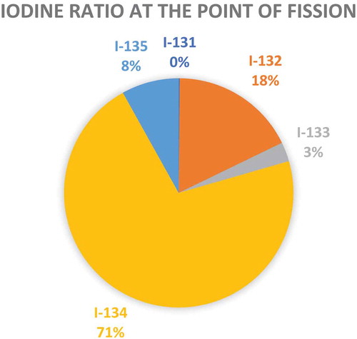
Table 16. 137Cs activities in soil and grass in India.
Table 17. Radionuclide ratio in workers at the Chernobyl accident.
Figure 23. The samplers used by MeGaw and May. On the left is the simple iodine vapour and particles filter. The bold line is the asbestos paper filter while the two normal vertical lines are the charcoal impregnated paper filters. On the right is the more complex device which can provide more details of the speciation of the iodine. The dotted vertical line is the Millipore filter (particles), the two blue vertical lines are the charcoal impregnated paper filters (elemental iodine) while the charcoal pad is used to capture iodine compounds.
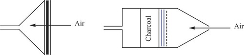
Figure 24. The improved “May Pack” from 1963. The device was improved by the addition of the copper gauzes (dotted red lines) which are in front of the Millipore filter.
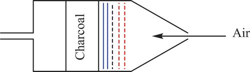
Figure 25. The first of the two improved May-Pack devices reported by Noguchi et al.
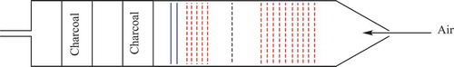
Figure 26. Prediction of the number of atoms of different nuclides with a mass of 89 in both the liquid and the headspace above a liquid.
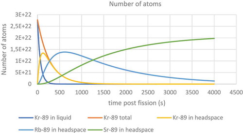
Figure 27. Prediction of the radioactivity associated with different nuclides with a mass of 89 in the liquid and the headspace.
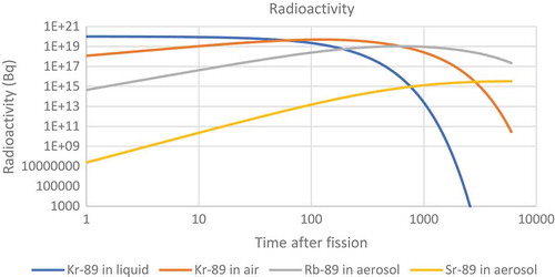
Figure 28. Prediction of the radioactivity of different nuclides with a mass of 91 in both the liquid and the headspace above a liquid.
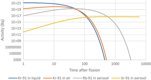
Figure 29. Prediction of the number of atoms of different nuclides with a mass of 91 in both the liquid and the headspace above a liquid.
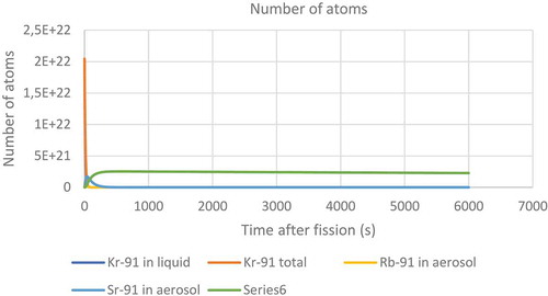
Table 18. Heats of formation.
Table 19. Details of rodent plutonium injection experiments.
Figure 30. The change in the radiotoxicity of the transuranium actinides released by Chernobyl.
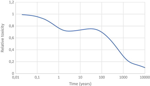
Figure 31. The relative contribution of plutonium, americium and curium to the radiotoxicity of transuranium elements released by Chernobyl.
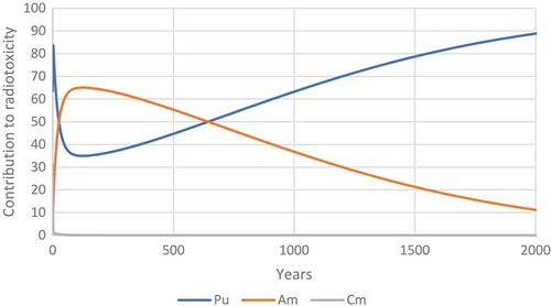
Figure 32. The relative contribution of plutonium, americium and curium to the radiotoxicity of transuranium elements released by Chernobyl.
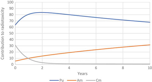
Table 20. Plutonium isotope signatures for Chernobyl and the Fukushima reactors.
Table 21. Activity ratios in the water samples from the basement of unit 4 of Chernobyl and the fuel.
Table 22. Details of radiotracers of the lanthanides.
Table 23. Details of europium and gadolinium isotopes.