
Figures & data
Figure 1. Examples of two CT axial slices with their corresponding simulated CBCT. The intensity profiles of the central row (marked as a line in both images) are plotted in the right panel. Each image is displayed with Window = 1300, Level = 0.
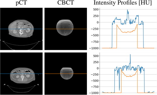
Figure 2. Schematic of the Generator model architecture.
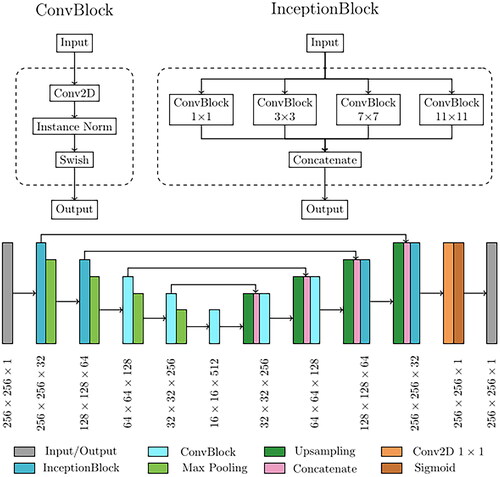
Figure 3. Schematic of sCT generation pipeline. *Rigid registration step is applied only to real CBCT scans since generated ones are intrinsically perfectly aligned.
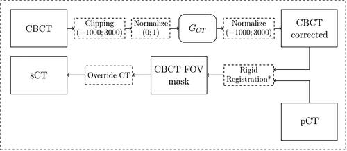
Figure 4. Example a CBCT axial slice before (left) and after (right) cGAN correction. As it can be noticed, the cGAN was effective in the correction of the CBCT. Each image is displayed with Window = 1300, Level = 0.
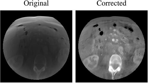
Figure 5. Examples of two CT axial slices with their corresponding sCT generated overriding the uncorrected simulated CBCT (sCTu) and the corrected ones (sCTc). The intensity profiles of the central row (marked as a line in both images) are plotted in the right panel. Each image is displayed with Window = 1300, Level = 0.
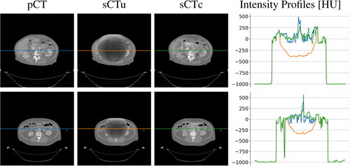
Figure 6. Performance metrics for cGAN model evaluation, computed on the axial slices of the test set before and after model processing.
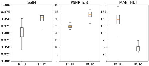
Figure 7. Example of dose planning for an axial slice of a subject for the original pCT, sCTu, and sCTc (upper row). The difference between both sCT treatment plans with respect to the original pCT plan is shown in the bottom row. Synthetic CT scans in this figure were produced using a simulated CBCT as the input.
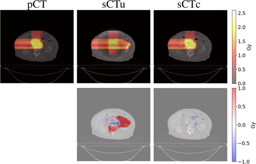
Figure 8. Example of DVH computed for ROI and two organs at risk (bowel and stomach). Solid line: pCT, dashed line: sCTu, dotted line: sCTc. Synthetic CT scans in this figure were produced using a simulated CBCT as the input.
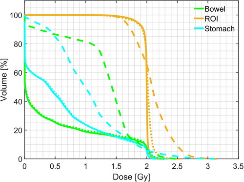
Table 1. Gamma pass rate results for different criteria computed using only the simulated CBCT dataset as input to the framework. Statistical difference in gamma score distributions, between uncorrected and corrected sCT, was found (p < 0.001).
Table 2. Mean doses, D5, and D95, measured on ROI, bowel, and stomach, computed using only the simulated CBCT dataset as input to the framework. Values are expressed as median(IQR) Gy.
Figure 9. Overlay of corrected CBCT (pink) on pCT (green) before (left) and after (right) rigid registration. It can be seen that the registration was effective in the alignment of the bony structures. Each image is displayed with Window = 1300, Level = 0.
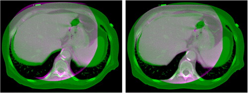
Figure 10. Example of dose planning for an axial slice of a subject for the original pCT, sCTu, and sCTc (upper row). The difference between both sCT treatment plans with respect to the original pCT plan is shown in the bottom row. Synthetic CT scans in this figure were produced using a real CBCT as the input.
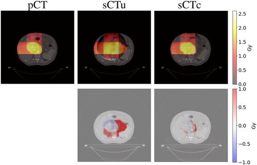
Figure 11. Example of DVH computed for ROI and two organs at risk (bowel and stomach). Solid line: pCT, dashed line: sCTu, dotted line: sCTc. Synthetic CT scans in this figure were produced using a real CBCT as the input.
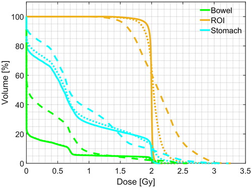
Table 3. Gamma pass rate results for different criteria computed using real CBCT dataset as input to the framework. Statistical difference in gamma score distributions, between uncorrected and corrected sCT, was found (p < 0.001).
Table 4. Mean doses, D5, and D95, measured on ROI, bowel, and stomach, computed using only the real CBCT dataset as input to the framework. Values are expressed as median(IQR) Gy.
Table 5. Comparison of dosimetry results with literature outcomes in terms of GPR2%/2 mm in the domain of proton therapy.
Data availability statement
The data presented in this study are openly available in The Cancer Imaging Archive (TCIA) at 10.7937/TCIA.ESHQ-4D90. These collections are freely available to browse, download, and use for commercial, scientific and educational purposes as outlined in the Creative Commons Attribution 3.0 Unported License.