Semiparametric Latent ANOVA Model for Event-Related Potentials

Figures & data

Figure 1. Simulation study. (Top) The ten simulated regression functions and corresponding curve fitting, for the first subject only, for group 1 with sine functions, and (Bottom) for group 2 with cosine functions. In the curve fitting plots, the light blue shaded area indicates the 95% credible interval for f(x), estimated from the sample paths ${\{{\widehat{f}}^{(d)}(x)\}}_{d=1}^D$ drawn from the posterior derivative Gaussian process, and corresponding to the sampled latencies ${\left\{{\mathbf{t}}^{(d)}\right\}}_{d=1}^D.$ The mean of those realizations is shown as the red dashed line, the green dashed fitted curve is obtained from the LOESS method, and the true f(x) is shown in blue color.

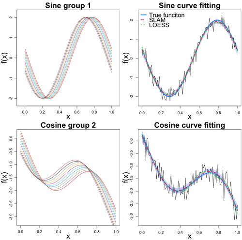
Figure 2. Simulation study: (Top) Latency estimates for group 1 with sine functions and (Bottom) for group 2 with cosine functions.

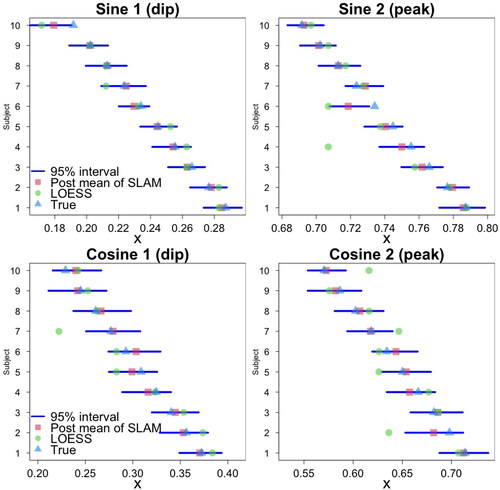
Figure 3. Simulation study: (Top) Posterior histograms of t of the sine regression function for the 8th subject. (Middle) Posterior distribution of group-level parameters r¹ and r² for the sine and cosine regression function settings. The blue vertical dashed lines indicate true subject-level latencies. The red segments are the 95% credible intervals from the posterior distributions by SLAM, and the black segments are the 95% confidence intervals using the two-step approach by fitting LOESS followed by one-way ANOVA. (Bottom) Amplitude distributions using the Max Peak method in Algorithm 2. Vertical red lines indicate the true amplitudes, and the green lines indicate the LOESS estimates.

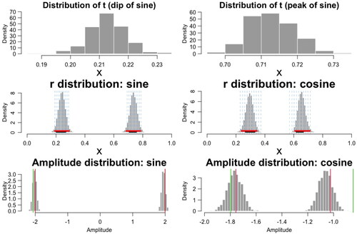
Figure 4. Simulation study: (Top) Examples of simulated regression functions and corresponding curve fitting, for the first subject only, for group 1 with sine functions, and (Bottom) for group 2 with cosine functions. There is a group-level stationary point in the region $(0,0.5)$ and in $(0.5,1).$ The black dashed line separates the two regions, and the red vertical lines indicate the true group-level latencies. The true f(x) is shown in blue color.

Figure 5. Case study: (Top) Subject-level ERP curves and grand average ERP curves. Solid: Young group. Dashed: Older group. The 0 ms time, which corresponds to time point 100, is the start of the onset of sound. The N100 component of interest is the dip characterizing the signal in the time window [60–140] ms colored in green. The P200 component characterizes the time window [140–220] ms, colored in yellow. (Bottom) Posterior distribution of subject-level latencies.

Figure 6. Case study: (Top) Latency difference between groups and latency shift effect on the right. (Bottom) Amplitude difference between groups.

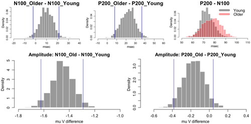
Table 1. Simulation study: Latency and amplitude comparison. Average and the standard deviations (in parentheses) of the RMSEs from the 100 replicated data sets.

	Latency
Method	Group 1: Sine	Group 2: Cosine
SLAM-posterior mean	0.0037 (0.0000)	0.0068 (0.0002)
SLAM-median	0.0036 (0.0001)	0.0068 (0.0002)
LOESS	0.0119 (0.0021)	0.0251 (0.0036)
	Amplitude
SLAM-posterior mean	0.0421 (0.0004)	0.0582 (0.0016)
SLAM-median	0.0421 (0.0005)	0.0581 (0.0016)
LOESS	0.0661 (0.0007)	0.0654 (0.0066)

Table 2. Simulation study: Parameter estimation. The mean and standard deviation of posterior mean and RMSE are computed from 50 replicates of data with size 100.

		Mean (SD) of posterior mean		Mean (SD) of RMSE
Parameter	True value	10 subjects	20 subjects	10 subjects	20 subjects
$r_1^1$	0.57	0.54 (0.033)	0.56 (0.027)	0.077 (0.016)	0.050 (0.012)
$r_1^2$	0.43	0.46 (0.028)	0.44 (0.024)	0.077 (0.012)	0.051 (0.011)
$r_2^1$	0.45	0.45 (0.035)	0.45 (0.029)	0.075 (0.010)	0.051 (0.009)
$r_2^2$	0.67	0.63 (0.033)	0.65 (0.025)	0.084 (0.017)	0.052 (0.010)
${\beta }_0^1$	0.3	0.17 (0.135)	0.24 (0.109)	0.314 (0.064)	0.205 (0.049)
${\beta }_0^2$	−0.3	−0.17 (0.114)	−0.24 (0.100)	0.317 (0.049)	0.210 (0.043)
${\beta }_1^1$	−0.5	−0.38 (0.276)	−0.44 (0.222)	0.463 (0.115)	0.319 (0.100)
${\beta }_1^2$	1	0.72 (0.244)	0.88 (0.203)	0.538 (0.127)	0.351 (0.093)
σ	0.5	0.57 (0.003)	0.57 (0.003)	0.074 (0.002)	0.074 (0.002)

Data Availability Statement

Behavioral and Event-Related Potentials data that support the findings in this paper are available on PsyArxiv Noe and Fischer-Baum (2020) at https://osf.io/c7k4s/ (DOI 10.17605/OSF.IO/C7K4S).