Figures & data
Figure 1. Simplified schematic diagram of a catheter-based ultrasound applicator composed of four axial transducers within an implant catheter (R is the radius of the catheter, Re is the radius of the transducer and Le is the length of the transducer). Each transducer can be circularly sectored to produce directional heating patterns; the sector angles applied herein include 360°, 180°, 270°, 2 × 180°, 120°, and 90° (arrows represent the direction of acoustic energy and heat delivery). The larger endocavity applicator can be dual-sectored. The parameters of the interstitial and endocavity applicators applied in this paper are listed.
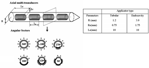
Figure 2. Examples of geometry planning and anatomy-based 3D thermal modeling of catheter-based ultrasound hyperthermia treatment using (a) an intrauterine applicator for cervix and (b) multiple interstitial applicators for prostate. CT scans (slice thickness 2.5 or 3 mm) were overlaid by segmented contours of rectum, bladder and target.
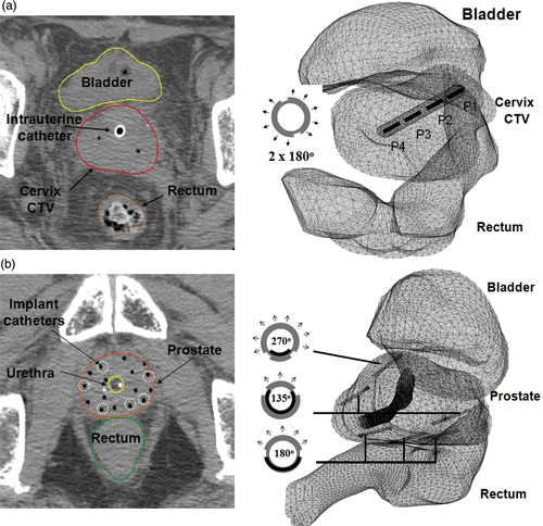
Table I. Acoustic and thermal parameters of tissue used for the treatment planning optimisation and simulations.
Figure 3. Optimised hyperthermia treatment plans calculated for GYN1, GYN2 and GYN1-GTV cases for intrauterine treatment of cervical cancer: the 3D geometry and anatomical models, temperature distributions, isothermal clouds (T ≥ 41°C) and isothermal dose clouds (t43 ≥ 10 min) are shown, using constraints of Tmax = 46°C and Ttargetmin = 42°C.
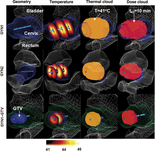
Figure 4. Thermal dose volume histograms (TDVH) and temperature volume histograms (TVH) for optimised treatment plans of intrauterine hyperthermia for cases GYN1, GYN2 and GYN1-GTV. The optimisations were carried out following the constraints as shown in the legend.
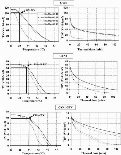
Table II. Summary of final optimised applied power levels for each GYN and prostate treatment plan (Tmax = 46°C, Ttargetmin = 42°C). Average values and the range from minimum to maximum are reported.
Table III. The maximum temperature and maximum thermal dose calculated within the surrounding rectum and bladder by the optimization-based treatment plans.
Table IV. Summary of the maximal width and length of the 41°C isothermal cloud and corresponding target volumes for the GYN and prostate cases.
Figure 5. Optimised hyperthermia treatment plans calculated for PROS1, PROS2 and PROS1-DIL cases for interstitial treatment of prostate target regions: the 3D geometry and anatomical models, temperature distributions, isothermal clouds (T ≥ 41°C) and isothermal dose clouds (t43 ≥ 10 min) are shown, using constraints of Tmax = 46°C and Ttargetmin = 42°C.
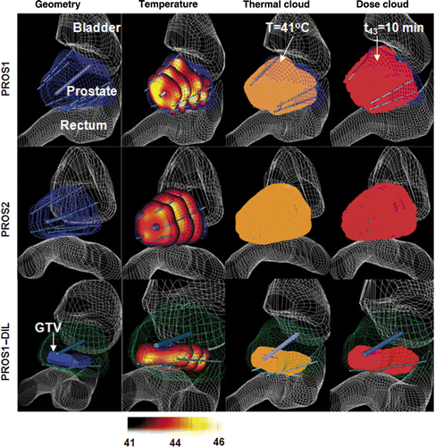
Figure 6. Thermal dose volume histograms (TDVH) and temperature volume histograms (TVH) for optimised treatment plans for optimised interstitial hyperthermia treatment of PROS1, PROS2 and PROS1-DIL cases. The optimisations were carried out following the constraints, in which the Tmax and Ttargetmin are listed in the legend.
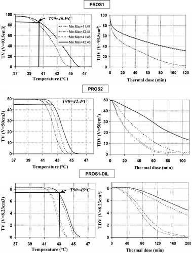
Figure 7. Precision and convergence of optimisation for GYN hyperthermia with different initial guesses. (a) The boxplot of optimised power values of two dual-sectored (2 × 180°) ultrasonic transducers for GYN-GTV, (b) the log-scaled convergence plot for optimisations starting with four different initial settings.
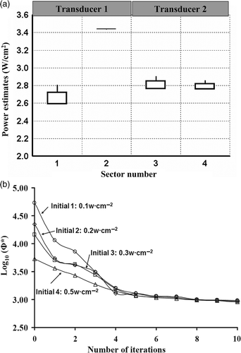
Figure 8. Precision and convergence of optimisation for prostate hyperthermia with different initial guesses. (a) The boxplot of optimised power values of six interstitial applicators with 24 ultrasonic transducers for PROS1, (b) the convergence plot for optimisations starting with four different initial settings.
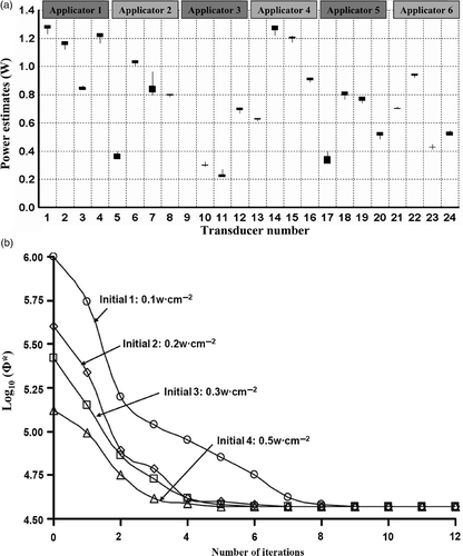
Figure 9. (a) Range of optimised applied power levels for 24 transducer sections on six applicators as calculated for different blood perfusion values (0.5–5 kg m−3 s−1) for treatment planning of PROS1; (b) Diagram demonstrating the relative positioning of the applicators, sequentially labelled a1through a6, and the corresponding transducers as indexed in (a). The transducer index of each applicator starts on the proximal end (towards the apex of the prostate) and increases toward the distal end (prostate base), with four transducers per applicator.
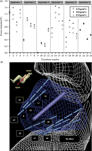
Table V. Summary of the computation time required to generate each optimised treatment plan, distinguishing between time for power optimisation and forward treatment simulation.
Table VI. The impact of changes in perfusion from nominal values, as used in the optimisation-based planning, on Tmax and T90 calculated within the target volume for the prostate and GYN test cases. Transducer power levels were optimised for a nominal perfusion (ω* = 2.5 kg m − 3 s−1), and applied for an increase (ω = 5 kg m−3 s−1) and a decrease (ω = 0.5 kg m−3 s−1) in perfusion values for comparative purposes.