Magnetic resonance temperature imaging validation of a bioheat transfer model for laser‐induced thermal therapy

Figures & data

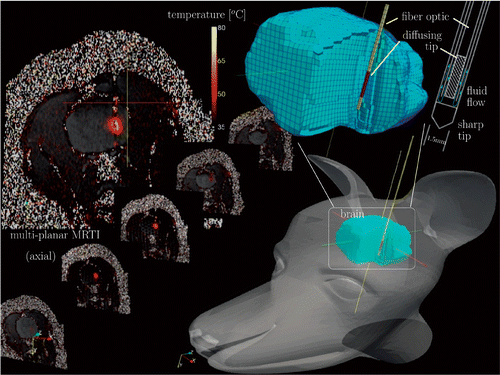
Figure 1. Schematic diagram of in vivo MR-guided LITT procedure in a canine model of brain. A 1.5-mm diameter water-cooled diffusing tip applicator was introduced percutaneously through the parietal bone. The applicator consisted of two clear, concentric tubes for water flow, the central of which contains an active 1-cm diffusing tip 400 µm diameter silica fibre-optic. Delivery of the photothermal energy is monitored using a multiplanar EPI sequence for MR temperature imaging.

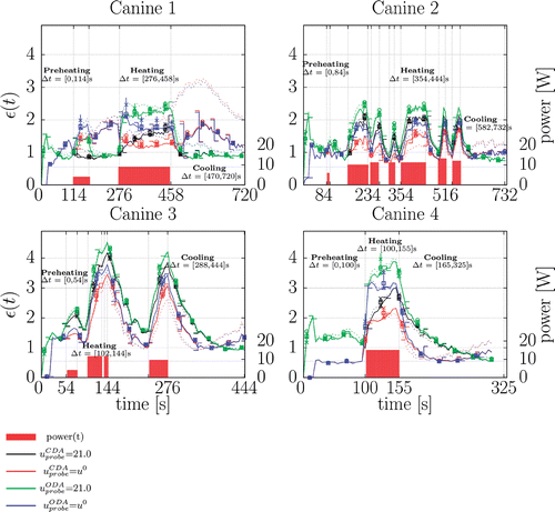
Figure 2. Normalised error history. The history of the L₂ error normalised by the measured multiplanar temperature image noise (4), ϵ(t), is shown for each canine in this study. The normalised error is dimensionless. Data is plotted at . The error bars shown provide the error range for the perfusion values considered; error bars left and right of the vertical axis plot , respectively. Dotted lines plot ω = 0.0 for comparison. Permutations of laser (CDA, ODA) and cooling model u_probe = (21°C, ) are shown for each canine. The power history of the thermal dose deliver is plotted against the right axis as a reference. Power is provided in W. The labelled time intervals highlight three regimes of interest: prior to heating, during heating, and during cooling. The corresponding pointwise maximum error plots during each of the regimes is provided for the centre plane of the multiplanar data in Figures 3–4. The -×-□-○-Δ sequence shown illustrates the convergence of the finite element numerical solution throughout the thermal dose history. The -×-□-○-Δ plots values of the error metric (4) at when monotonically increasing the mesh resolution (decreasing element diameter from 2 mm to 0.5 mm).

Table 1.  Constitutive data [9], [23], [24]

		g
0.527	0.0, 3.0, 6.0, 12.0	0.862	47.0	0.45	1045	3840	3600

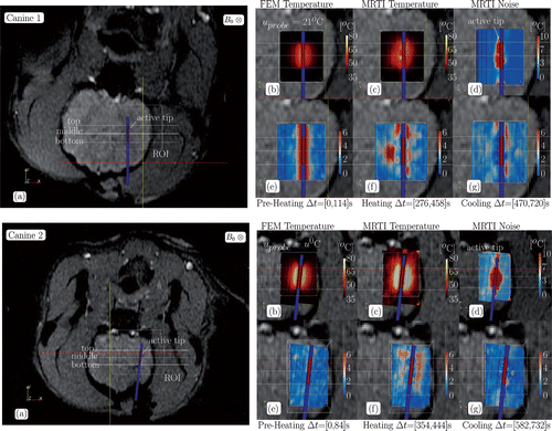
Figure 3. Canine 1-2 data summary, CDA, (a) The anatomical position of the ROI and the spatial profiles used in Figure 5 are illustrated on magnitude images of the anatomy. Cutplanes through the ROI of the finite element data used in Figure 2 is shown in (b–g). Cutplanes are coplanar with the applicator. The pointwise maximum over time for the (b) FEM predicted temperature, (c) MR temperature data, and (d) MR temperature noise is provided in °C. The pointwise maximum normalised error (5) over time for the (e) pre-heating, (f) heating, and (g) cooling regimes labelled in Figure 2 are provided.

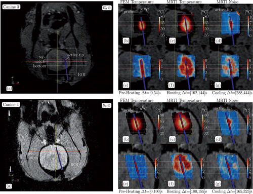
Figure 4. Canine 3-4 data summary, CDA, (a) The anatomical position of the ROI and the spatial profiles used in Figure 5 are illustrated on magnitude images of the anatomy. Cutplanes through the ROI of the finite element data used in Figure 2 are shown in (b–g). Cutplanes are coplanar with the applicator. The pointwise maximum over time for the (b) FEM predicted temperature, (c) MR temperature data, and (d) MR temperature noise is provided in °C. The pointwise maximum normalised error (5) over time for the (e) pre-heating, (f) heating, and (g) cooling regimes labelled in Figure 2 are provided.

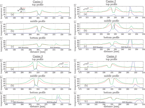
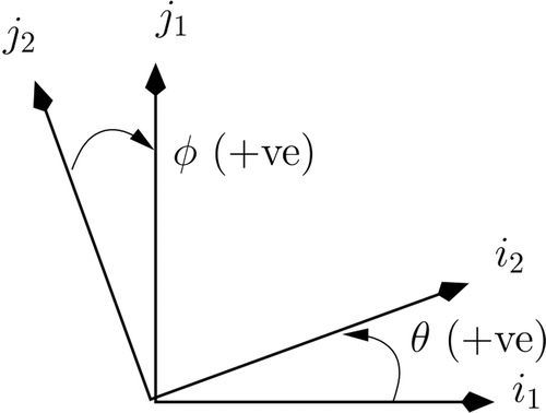
Figure 5. Canine 1-4 spatial profiles summary, CDA, The (a) top, (b) middle, and (c) bottom profiles illustrated in Figures 3, 4(a) plot the maximum over time of the MR temperature data (°C), computational prediction (°C), and MR temperature noise (°C) against distance (mm). Profiles extend beyond the ROI used in normalisation in Figure 2; the boundary of the ROI is denoted on the profiles.

Figure 6. Polar convention.

Pennes HH. Analysis of tissue and arterial blood temperatures in the resting forearm. J Appl Physiol 1948; 1: 93–122

 PubMed Web of Science ®Google Scholar

Fuentes D, Feng Y, Elliott A, Shetty A, McNichols RJ, Oden JT, Stafford RJ. Adaptive real-time bioheat transfer models for computer driven MR-guided laser induced thermal therapy. IEEE Trans Biomed Eng 2010; 57

 PubMed Web of Science ®Google Scholar

Arkin H, Xu LX, Holmes KR. Recent developments in modeling heat transfer in blood perfused tissues. IEEE Trans Biomed Eng 1994; 41: 97–107

 PubMed Web of Science ®Google Scholar