Figures & data
Table I. Material properties used in biothermal models.
Figure 1. (A) Diagram of the ultrasound applicators modelled. Blue arrows indicate the direction of cooling flow, which runs through the centre of the applicator, out the tip, and then between the applicator and the catheter. Transducers have an outer diameter of 1.5 mm. The catheter has an outer diameter of 2.4 mm and an inner diameter of 1.89 mm. A convective boundary condition is applied to the inner wall of the catheter. (B) Geometry used to model interstitial ultrasound ablation with the applicator at various distances (0.5 cm < d < 3.2 cm) from the surface of a flat bone.
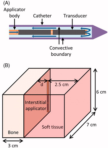
Figure 2. Ultrasound reflection and refraction at bone/soft tissue interfaces, as used to derive the models herein. An incident wave strikes the bone surface at angle and intensity I. The reflected wave, refracted longitudinal wave, and refracted shear wave have intensities R, TL, and TS and travel at angles
,
, and
, respectively.
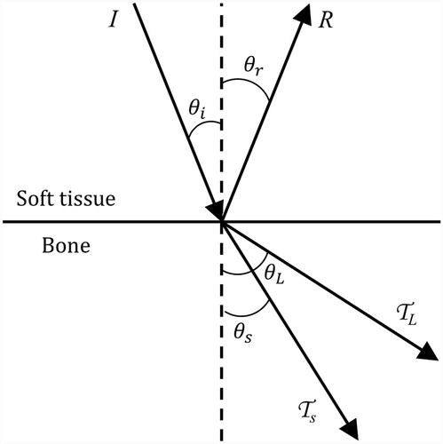
Table II. Properties of the four types of models.
Figure 3. Set-up of ex vivo bench-top experiments. (A) In experiments with ex vivo muscle and bone, a cut of porcine muscle was placed on top of bovine bone and heated. (B) In phantom and ex vivo bone experiments, the temperature rise in a phantom with an encapsulated bone was measured by thermocouples within needles.
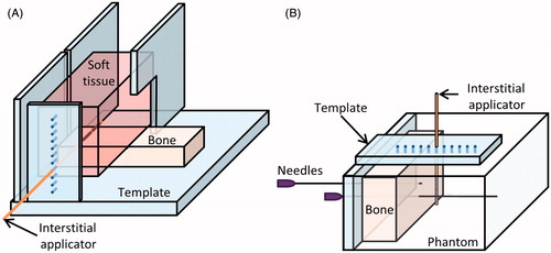
Figure 4. 240 CEM43 °C contours calculated with models A–D after a 10-min ablation are shown in the central plane between the two transducers. The applicators (white circle) are placed 1 and 2 cm from a flat bone (black line) in A and B, respectively. A colour map shows the temperatures (°C) calculated with the constant transmission volumetric model (model B).
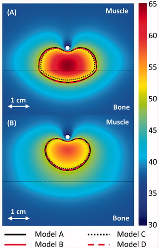
Figure 5. The maximum distance between an applicator and a flat bone at which all tumour tissue between the two can be ablated within 10 min, given various ultrasound attenuations and blood perfusion rates in the tumour, as calculated by model B. The maximum radius that can be fully ablated when bone is absent is also shown for 0 and 13 kg/m3/s perfusion in the tumour. The maximum distance between an applicator and bone for which all intervening tissue can be ablated is also plotted for models A (+), C (o), and D (Δ) for attenuations of 4 and 12.5 Np/m/MHz and perfusions of 0 (black), 5 (red), and 13 (blue) kg/m3/s.
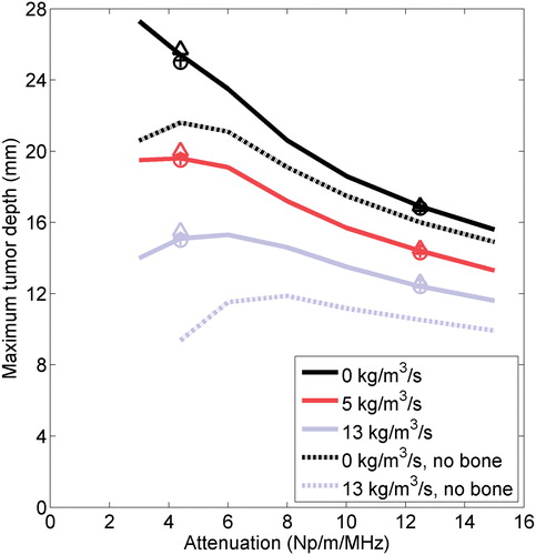
Figure 6. (A–C) Thermal lesions created by 10-min ablations at 12.5 acoustic W/cm2 in porcine muscle positioned directly atop bovine bone, shown in central cross-sections through the lesions. The catheter was measured as 15.2, 19.7, and 32.3 mm away from the bone before heating in A–C respectively, and 11.5, 17, and 32 mm away from the bone after the experiment. The catheter track is circled, and the side of the tissue that was against the bone is shown against the table. In C, a metal rod illustrates the catheter position. (D–F) The experiments were modelled with the applicator 15, 20, and 32 mm away from the bone, respectively, and the results after a 10-min ablation are plotted in the central plane between the two transducers. The resulting temperature profiles produced by model A are shown in a colour map (°C). A black line indicates the bone/muscle boundary, and curves outline the 52 °C temperature contours for models A–D.
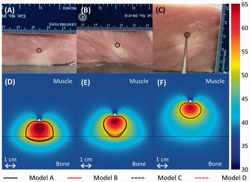
Figure 7. Experimental (---) and simulated (– – –) temperature profiles after 10-min ablations in two phantoms containing cortical (A) or cancellous (B) bone. Temperature along a line perpendicular to the bone surface and adjacent to the centre of one transducer, as in , is plotted as a function of distance from the bone surface, which is at x = 0. Positive x-values are in the phantom, and negative values are inside the bone. Each solid curve corresponds to a single experimental trial with the applicator placed at the designated distance from the bone. The experiments were simulated with model B, and the theoretical results are superimposed as dashed lines.
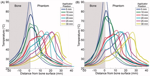
Figure 8. The maximum temperature increase measured at the end of each 10-min ablation of a phantom with an embedded bone is plotted in A. The temperature increase at the bone surface at the end of each trial is plotted in B. Peak (A) and bone (B) temperature increases produced by simulations using the constant transmission longitudinal model (model B) are superimposed.
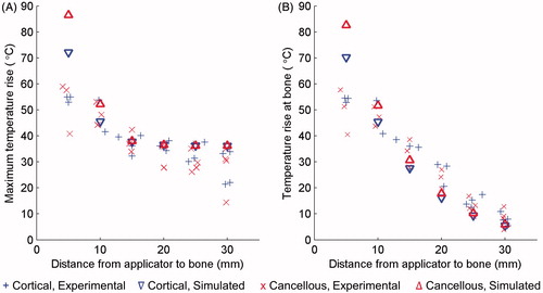
Figure 9. Simulated and experimental temperature profiles in phantoms with an applicator placed 10 mm (A) and 25 mm (B) from a rib surface. Temperature along a line perpendicular to the bone surface and adjacent to the centre of one transducer, as in , is plotted as a function of distance from the bone surface, which is at x = 0. Recordings were made after 10 min of heating. The experimental curve is an average of the recordings in three to four experiments with the applicator at the given position. The bone surface is at x = 0. Positive x-values indicate locations in the phantom, and negative values are inside the bone.
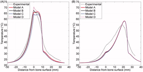
Table III. Correlation coefficients between experimental and simulated temperature profiles in phantoms.
Figure 10. 3D objects that were meshed to model the bovine vertebra (A) and bovine rib (B) ablations monitored by MR thermometry.
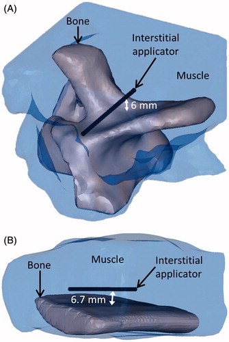
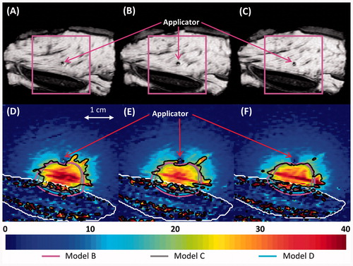
Figure 11. (A–C) MR images of the three central heated axial slices of ex vivo bovine vertebrae, spaced 5 mm apart. (D–F) Colour map of temperature increases (°C) recorded with MRTI in a smaller field of view (magenta box) for each slice 5 min into the ablation. Bone is outlined with a white line, and the 20 °C temperature increase contours recorded by MRTI are outlined in black. Also shown are the simulated 20 °C temperature increase contours produced by models B (magenta), C (grey), and D (blue).
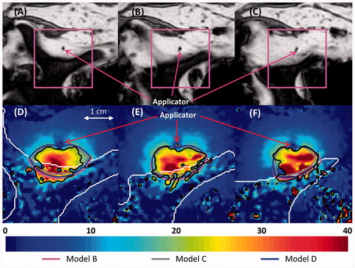
Figure 12. (A–C) MR images of the three central heated axial slices of ex vivo bovine rib, spaced 5 mm apart. (D–F) Colour map of temperature increases (°C) recorded with MRTI is shown in a smaller field of view (magenta box) for each slice 5 min into the ablation. Bone is outlined with a white line, and the 20 °C temperature increase contours recorded by MRTI are outlined in black. Also shown are the 20 °C temperature increase contours produced by models B (magenta), C (grey), and D (cyan).