Radiofrequency ablation lesion detection using MR-based electrical conductivity imaging: A feasibility study of ex vivo liver experiments

Figures & data

Figure 1. Experimental set-up for ex vivo liver RF ablation using MREIT. (A) RF ablation procedure in the bovine liver. (B) Top and side views of a conductivity phantom including the ablated liver block. (C) Four carbon-hydrogel electrodes are attached on the middle of the cylindrical surface to inject currents I₁ and I₂ along two different directions.

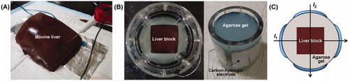
Figure 2. Typical MREIT images of normal liver tissue before RF ablation. (A, B) T1-, T2-weighted MR images of a liver tissue. (C) A magnetic flux density image induced by the horizontal injection current. (D, E) Reconstructed conductivity and colour-coded conductivity images of normal liver tissue. (F) Photograph of normal liver tissue at the same imaging slice. The conductivity images of normal liver tissue show a relatively lower homogeneous distribution compared to surrounding agar material. The white arrows indicate the ion diffusion and chemical reactions between the liver tissue and agarose gel.

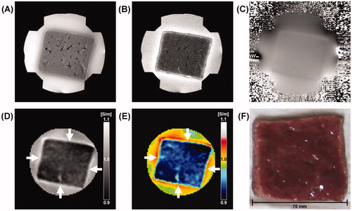
Figure 3. Typical MREIT images of ablated liver tissue with a power of 50 W following 3 min of exposure time. (A, B) T1-, T2-weighted MR images of ablated liver tissue. (C) A magnetic flux density image induced by the horizontal injection current. (D, E) Reconstructed conductivity and colour-coded conductivity images of ablated liver tissue showing a significantly increased contrast and well-defined lesions. (F) A photograph of ablated liver tissue at the same imaging slice. The arrows indicate the coagulation necrosis (white arrow) and the hyperaemic rim (black arrow).

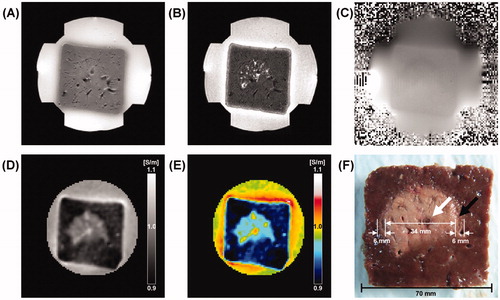
Table I. Relative conductivity contrast ratios (%) of liver tissues after RF ablation. Ablation lesions were created in a linear interrupted fashion using a power-controlled mode at 30, 50, and 70 W for 1, 3, and 5 min of exposure time, respectively.

	Power of 30 W				Power of 50 W				Power of 70 W
	1 min	3 min	5 min	pKW†, correlation§	1 min	3 min	5 min	pKW†, correlation§	1 min	3 min	5 min	pKW†, correlation§
Coagulation necrosis	0.31 ± 0.10	1.42 ± 0.20	2.43 ± 0.30	<0.001, 0.944	0.70 ± 0.15	3.07 ± 0.29	3.51 ± 0.36	<0.001, 0.867	3.69 ± 0.31	3.28 ± 0.40	3.02 ± 0.29	0.007, −0.704
Hyperaemic rim	0.26 ± 0.09	1.22 ± 0.22	1.58 ± 0.35	0.001, 0.853	0.53 ± 0.17	2.36 ± 0.42	2.80 ± 0.30	0.001, 0.834	2.84 ± 0.31	3.47 ± 0.19	3.63 ± 0.36	0.003, 0.713
pMW*	0.165	0.128	0.002		0.097	0.007	0.004		0.001	0.318	0.004

Notes: rCCRs of RF ablation lesion are mean ± standard deviation.

*pMW (Mann-Whitney test) was obtained from the comparison between the coagulation necrosis and hyperaemic rim.

†pKW (Kruskal-Wallis test) was obtained from the comparison among 1, 3, and 5 min of exposure times.

§Spearman correlation coefficient at the level of p < 0.01.

Figure 4. Time-course variation of liver tissue before and after RF ablation at 50 W. (A) T1-weighted, (B) T2-weighted, (C) reconstructed conductivity, and (D) colour-coded conductivity images obtained before and after 1, 3, and 5 min ablation time, respectively. Reconstructed conductivity images show significantly increased contrast and well-defined lesions for more than 3 min of exposure time.

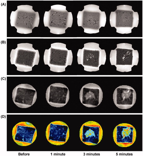
Figure 5. Power-dependent variation of liver tissue before and after RF ablation with the same exposure time of 5 min. (A) T1-weighted, (B) T2-weighted, (C) reconstructed conductivity, and (D) colour-coded conductivity images from the ablation lesions using a power-controlled mode at 30, 50, and 70 W, respectively. Reconstructed conductivity images show significantly increased contrast and well-defined lesions in all cases. The arrow indicates the charred tissue caused by thermal injury.

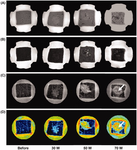
Figure 6. The bar graph shows the relative conductivity contrast ratio (%) of liver tissues by different exposure times and RF powers after RF ablation. Based on the conductivity value of normal liver tissue, the average rCCR of ablation lesion obtained from a total of seven liver blocks.

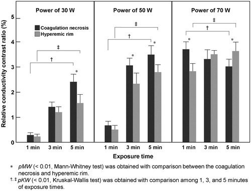
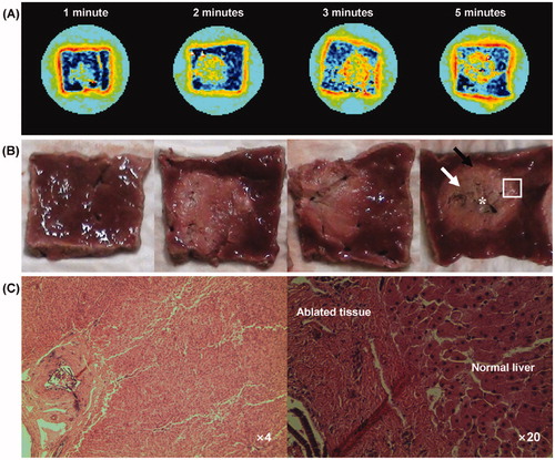
Figure 7. (A) Colour-coded conductivity images at the RF power of 70 W for 1, 2, 3 and 5 min of exposure time, respectively. (B) Photography shows the cross-section of ablated liver tissue at the corresponding conductivity imaging slice. The arrows indicate the carbonisation (asterisk), coagulation necrosis (white arrow) and the hyperaemic rim (black arrow). (C) Microscopic findings of ablated liver tissue obtained from the rectangle region (H&E stain, ×4 and ×20).