Figures & data
Figure 1. Schematic (left) and picture (right) of animal positioning for the experiment. The neck of the pig sits on top of a water bag used as coupling medium. Two multi-element surface coils are used for MRI acquisition. A moulding made with a foaming agent is used to immobilise the pig for the procedure.
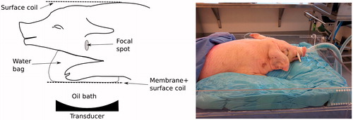
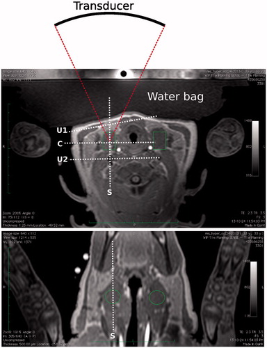
Figure 2. Transverse (top) and coronal (bottom) T1-weighted images of the target region in the pig’s neck. Muscle in the middle section on the right side of the neck was targeted for the treatment. Transverse image also shows the location of the transducer related to the target zone and water bag used for coupling. Locations of the monitoring stacks are also shown where ‘C’ and ‘S’ refer, respectively, to the coronal and sagittal views at focus, and ‘U1’ and ‘U2’ refer, respectively, to the user-defined stacks used to monitor pre-focal and post-focal heating.
Table
Figure 3. Example flowchart for thermometry using the look-up table (LUT) for the exhalation phase. (A) During pre-filling time tP), each new phase image (and a baseline temperature map) is stored in the LUT where its index is the normalised position (NDp, in %) in the breathing phase. (B) At the end of pre-filling (t = tP), the LUT is updated with phase maps that are linearly interpolated between 0 and 100%. (C) After pre-filling (tP), when a new image arrives the closest entry in the LUT is located according to NDp. The phase difference map is calculated between the phase maps of the new image and the best entry in the LUT. An updated thermal map is calculated with this phase difference map and the thermal map associated to the closest entry in the LUT. The updated thermal map is associated to the new phase map and both are inserted in the LUT as new entries.
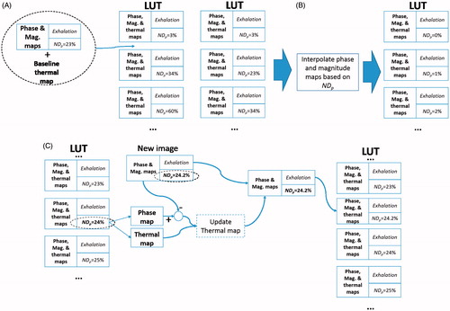
Table 1. Parameters values tested for multi-baseline correction.
Figure 4. Navigator profiles for hyperthermia experiments: (A) low displacement, (B) medium displacement and (C) high displacement. The raw unfiltered navigator displacement estimate is shown along the classified profile where legends M-less, Inh and Exh correspond, respectively, to motionless inhalation and exhalation.
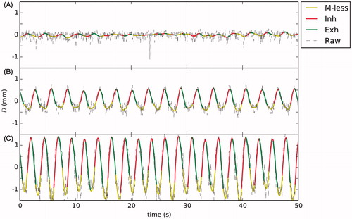
Figure 5. Logarithmic plots of the predicted trend of Spp (top row), SDC (middle row) and SppSDC (bottom row) using general additive modelling for the hyperthermia experiment with D = 1 mm. The selected plots are shown as functions of the duration to keep images stored in the LUT (tL), the pre-filling time (tP) and the number of interpolated images (nL) for the optimal conditions that minimised values of Spp,SDC and Spp SDC.
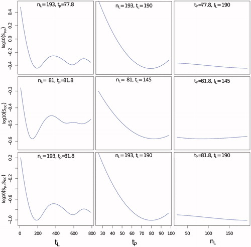
Table 2. Optimal values for execution of respiration compensation algorithm using multi-baseline correction. The values of SppSDC are shown for the fitted regression analysis with the global additive model (GAM), and calculated with and without the respiration compensation (RC) algorithm. The average (± SD) values of the resulting TSA-pp and TSA-DC are also shown.
Figure 6. Detail of spatial average temperature TSA (°C) over time on each of three ROIs and slice stacks (coronal and sagittal at focus, and two user-defined stacks) at the beginning of the hyperthermia experiments. Temperature is shown with and without respiration compensation by ‘–’ and ‘°’, respectively. Fibre-optic thermometer reading is shown by ‘…’. The baseline temperature at the beginning of treatment was subtracted. This baseline was 39 °C, 35.7 °C and 33.7 °C for Dpp values of 0.2 mm, 1 mm and 3 mm, respectively.
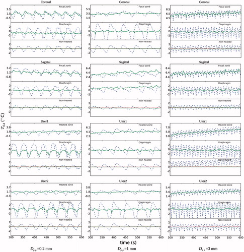
Figure 7. Detail of spatial average temperature TSA (°C) over time on each of three ROIs and slice stacks (coronal and sagittal at focus, and two user-defined stacks) at the end of the hyperthermia experiments. Temperature is shown with and without respiration compensation by ‘- -’ and ‘°’, respectively. The baseline temperature at the beginning of treatment was subtracted. A change of body temperature was observed in the fibre-optic thermometer readings, especially for the experiment with Dpp = 3 mm. For that experiment it is also worth noting that MRI temperature for the global non-heated region in the ‘User 1’ stack had a TSA-DC of 16 °C when no respiration compensation was applied, which meant that it was not plotted.
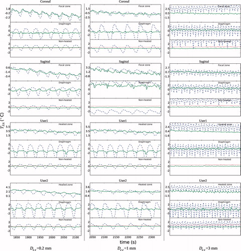
Figure 8. Comparison of temperature and thermal dose profiles for the hyperthermia experiment with D = 3 mm for treatment at ROI on the coronal plane with and without respiration compensation (RC). Profiles over time (top row) are shown for the average, T90 (above 10% percentile) and T10 (above 90% percentile) values on the treatment ROI. Maps of the average temperature (middle row) were calculated during the steady state of the treatment (between 500 s and 2000 s). Maps of the total accumulated thermal dose (bottom row) are shown in log10 scale. The treatment ROI is shown in both temperature and thermal dose maps by a circular zone of 8 mm of radius.
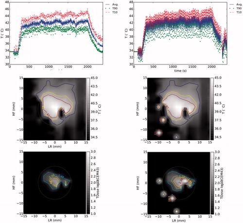
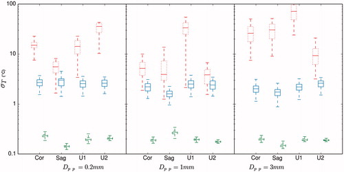
Figure 9. Box-plot of the variation of standard deviation of temperature σT on the non-heated region for each experiment and for the monitored coronal (Cor), sagittal (Sag) and user specified (U1 and U2) imaging stacks. σT is shown without and with respiration compensation by ‘…’ and ‘—’. The theoretical optimal value of σT is shown by ‘- -’. The margins in the boxes represent the median and the values of σT that comprise 25% and 75% of all data points. The bar limits show the extreme values that are exceeded by 10% and 90% of all data.