Figures & data
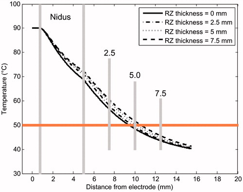
Figure 1. (a) Cortical osteoid osteoma consisting of a nidus surrounded by cortical and trabecular bone. The RF applicator is introduced into the nidus through a drill hole prior to RF application. (b) Theoretical model of cortical OO consisting of a nidus enclosed by a reactive zone.
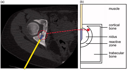
Figure 2. Relative positions of the OO and the cortical bone layer. We defined three directions in which temperature profiles were computed: −45°, 0° and 45° (origin at the midpoint of the electrode surface). Note that in Position 2, the 45° direction, has muscle tissue outside the reactive zone, while 0° and −45° have trabecular muscle. The intersection points between these directions and the outer layer of the reactive zone defined three locations at which the temperature was assessed (T45, T0 and T−45).
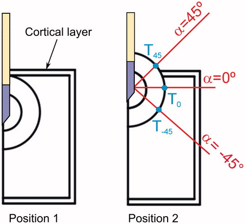
Table 1. Physical properties of the materials used in the model.
Figure 3. Maximum temperatures reached after 300 s of RFA at the outer limit of the reactive zone, in particular in the interface with trabecular bone (T0) and with muscle (T45) for different values of perfusion coefficient of nidus (ωn) and reactive zone (ωrz) (a, b), and of electrical conductivity of nidus (σn) and reactive zone (σrz) (c, d). A total of 64 simulations were conducted for each specific value of one of these parameters, varying the other three parameters (four values within a range). We then calculated and plotted the mean value of the 64 simulations. The maximum value of the difference with respect to the mean value was also plotted as a dispersion bar. These simulations were conducted with the OO in Position 2 (see ).
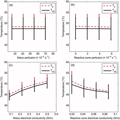
Figure 4. Temperature profiles (at 300 s) computed in the 0° direction (see ) for different electrical conductivity values of the reactive zone (a) and nidus (b). The 50 °C line represents the thermal lesion contour. These simulations were conducted with the OO in Position 2 (see ).
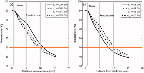
Figure 5. Distributed heat source qRF due to RF power in the involved tissues for different values of electrical conductivity of reactive zone σrz (a) and nidus σn (b). These simulations were conducted with the OO in Position 2 (see ).
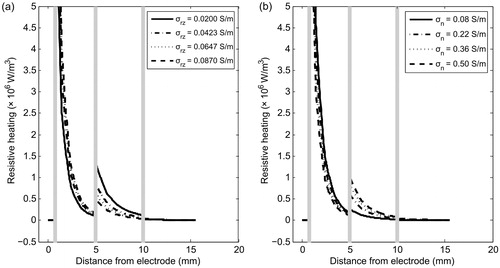
Figure 6. Progress of the applied voltage throughout RF ablation for different values of electrical conductivity of the reactive zone σrz (a) and nidus σn (b). These simulations were conducted with the OO in Position 2 (see ).
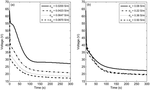
Figure 7. Temperature distributions (in °C) after 300 s of RFA for three RZ thicknesses: 2.5 mm (a), 5.0 mm (b) and 7.5 mm (c). Dashed line is the 50 °C isoline which represents thermal lesion contour. Progress of the thermal lesion radius throughout 300 s of RFA at the outer limit of the reactive zone for three RZ thicknesses: 2.5 mm (d), 5.0 mm (e) and 7.5 mm (f), and for three directions (α = 0, 45° and −45°). These simulations were conducted with the OO in Position 1 (see ).
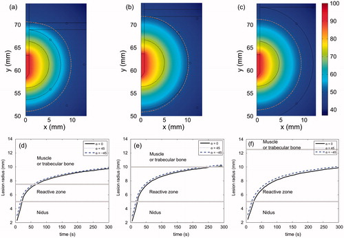
Figure 8. Effect of electrical conductivity of nidus (σn) and reactive zone (σrz) on electrical impedance (Ω) registered at the start of RFA. The effect of RZ thickness and OO position are also considered. Black and red colours correspond with Positions 1 and 2, respectively. Trend lines have been added as a guide.
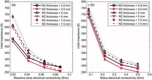
Table 2. Electrical impedance (Ω) at the start of RFA for different RZ thickness and electrical conductivity (σrz).
Table 3. Electrical impedance (Ω) at the start of RFA for different RZ thickness and electrical conductivity of the nidus (σn).
Figure 9. Temperature profiles (at 300 s) computed in 0° direction (see ) for different RZ thicknesses. The case without a reactive zone is also plotted (solid line). The 50 °C line represents the thermal lesion contour. All simulations were conducted with OO in Position 1 (see ).