Simulation of non-linear acoustic field and thermal pattern of phased-array high-intensity focused ultrasound (HIFU)

Figures & data

Figure 1. Illustration of step-marching scheme and second-order operator splitting operator used in the nonlinear acoustic wave propagation plane-by-plane in incremental steps from the transducer. Each step involves the effect of diffraction (D), attenuation (A), and nonlinearity (N).

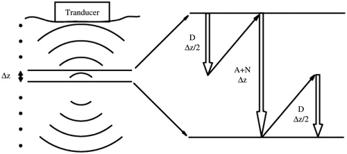
Figure 2. Schematic diagram of (a) a 331-element concave phased-array HIFU transducer and (b) the 3 layered media model used in the simulation.

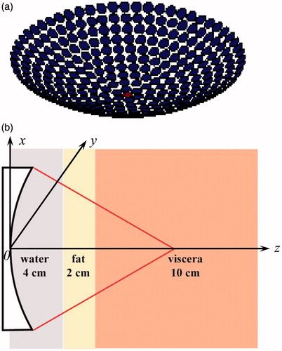
Figure 3. Comparison of the first 5 harmonics on the axis of the HIFU transducer using the KZK equation (solid line) and the angular spectrum approach with second-order operator splitting scheme (dashed line) in a two layered media model.

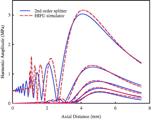
Table 1. Acoustic parameters of different media used in the simulation.

	Water	Tissue	Fat	Viscera
Density ρ	1000 kg/m^3	1050 kg/m^3	950 kg/m^3	1060 kg/m^3
Speed of sound c	1500 m/s	1629 m/s	1460 m/s	1540 m/s
Non-linearity β	3.5	4.5	6.5	4.7
Attenuation α0	0.025 Np/m/MHz^b	6.68 Np/m/MHz^b	15 Np/m/MHz^b	3.2 Np/m/MHz^b
Attenuation law b	2	1.3	1.0	1.25

Figure 4. Comparison of the pressure waveforms at the focus of an annular HIFU transducer measured by a needle hydrophone and numerical simulations using the 2nd order operator splitting algorithm and the KZK model.

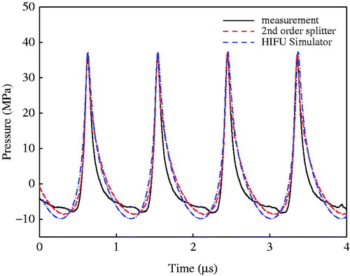
Figure 5. Comparison of the first 3 harmonics distribution (a) along and (b) transverse to the transducer axis obtained from the measurement and simulations using the 2^nd order operator splitting algorithm and the KZK model.

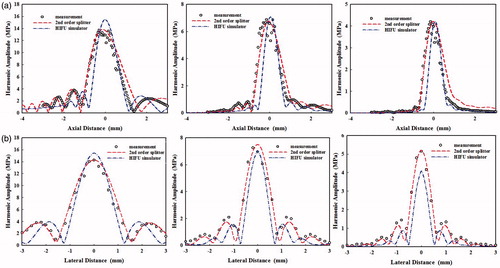
Figure 6. The simulated harmonics generated by the phased-array transducer in water with an input acoustic intensity of 8.33 W/cm² along the axial axis (left column) and the lateral axis (middle column), and the pressure waveform at the focus (right column) with different focusing strategies: (a) geometrically focusing at (0, 0, 10) cm, (b) transverse focus shifting at (1, 0, 10) cm, and (c) generation of four foci at (−1, −1, 10) cm, (−1, 1, 10) cm, (1, −1, 10) cm, (1, 1, 10) cm.

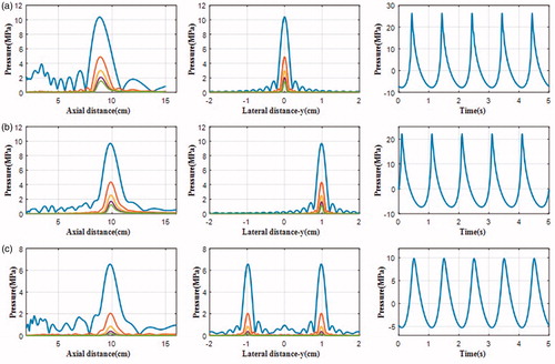
Figure 7. The simulated harmonics generated by the phased-array transducer in three layer media model with an input acoustic intensity of 8.33 W/cm² along the axial axis (left column) and the lateral axis (middle column), and the pressure waveform at the focus (right column) with different focusing strategies: (a) geometrically focusing at (0, 0, 10) cm, (b) transverse focus shifting at (1, 0, 10) cm, and (c) generation of four foci at (−1, −1, 10) cm, (−1, 1, 10) cm, (1, −1, 10) cm, (1, 1, 10) cm.

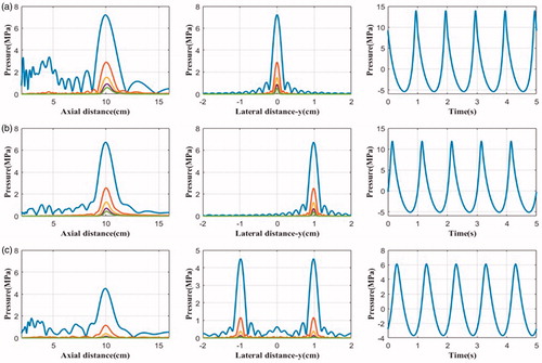
Table 2. Comparison of acoustic pressure at the focal points in water and tissue generated by different focusing patterns.

	p^+ (MPa)		p^- (MPa)		Grating lobe (dB)
	Water	Tissue	Water	Tissue	Water	Tissue
On-axis focus	27.05	13.67	7.33	5.02	−23.03	−15.5
Off-axis focus	23.97	12.33	6.95	5.00	−21.86	−14.26
Four foci	10.09	6.11	5.01	3.58	−18.46	−10.62

p⁺ peak positive pressure; p^- peak negative pressure.

Figure 8. The simulation distribution of fundamental harmonic (left column), 2^nd harmonic (middle column) and 3^rd harmonic (right column) in the x-z plane generated by the phased-array transducer in three layer media model with an input acoustic intensity of 8.33 W/cm² with different focusing strategies: (a) geometrically focusing at (0, 0, 10) cm, (b) transverse focus shifting at (1, 0, 10) cm, and (c) generation of four foci at (−1, −1, 10) cm, (−1, 1, 10) cm, (1, −1, 10) cm, (1, 1, 10) cm.

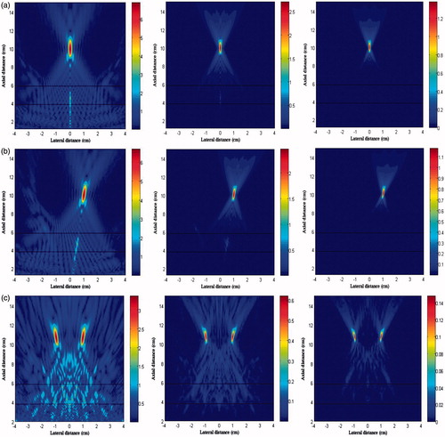
Figure 9. The simulation distribution of (a) peak positive pressure and (b) peak negative pressure in the x-z plane generated by the phased-array transducer in three layer media model with an input acoustic intensity of 8.33 W/cm² with different focusing strategies: geometrically focusing at (0, 0, 10) cm (left column), transverse focus shifting at (1, 0, 10) cm (middle column), and generation of four foci at (−1, −1, 10) cm, (−1, 1, 10) cm, (1, −1, 10) cm, (1, 1, 10) cm (right column).

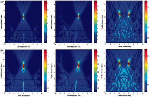
Figure 10. Comparison of the thermal field in the x-y plane (left column) and x-z plane (middle column) and presence of grating lobes in the x-z plane (right column) after 2-second continuous HIFU ablation through three layered media with an input acoustic intensity of 8.33 W/cm² using different focusing strategies (a) geometrically focusing at (0, 0, 10) cm, (b) transverse focus shifting at (1, 0, 10) cm, and (c) generation of four foci at (−1, −1, 10) cm, (−1, 1, 10) cm, (1, −1, 10) cm, (1, 1, 10) cm.

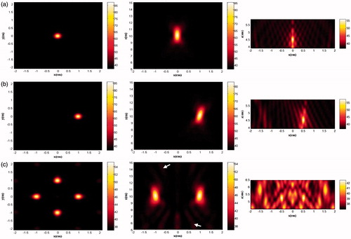
Figure 11. Comparison of the temperature elevation at the focal point during 2-second continuous HIFU ablation using different focusing strategies simulated by linear (solid line) and nonlinear acoustic model (dash line).

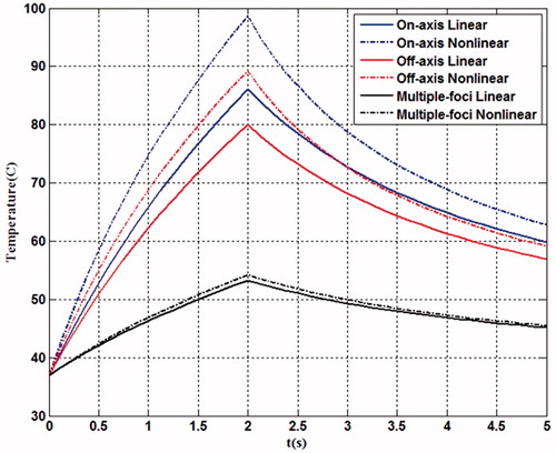
Figure 12. Comparison of the lesion size in (a) x-y plane and (b) x-z plane using different focusing strategies predicted by the linear (solid line) and nonlinear (dashed line) acoustic model after 2-second continuous HIFU ablation through three layered media with an input acoustic intensity of 8.33 W/cm².

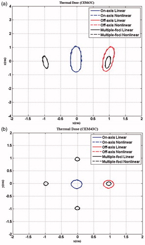
Table 3. Comparison of the maximum temperatures at the focal points after 2 s HIFU ablation and the lesion size in the tissue generated by different focusing patterns using linear and non-linear models.

	Maximumtemperature (°C)		Lesion area xz (mm^2)		Lesion area xy (mm^2)		Lesion volume (mm^3)
	Non-linear	Linear	Non-linear	Linear	Non-linear	Linear	Non-linear	Linear
On-axis focus	98.7	86.1	53.7	48.8	8.9	8.2	126.6	111.3
Off-axis focus	89.3	80.0	47.6	43.9	7.7	7.3	103.9	93.1
Four foci	54.2	53.2	∼12.5	∼11.3	∼1.95	∼1.83	47.2	42.8

Table 4. Comparison of the maximum temperatures at the focal points and in the pre-focal grating lobes after 2 s HIFU ablation and the lesion size in the tissue generated by different focusing patterns when adjusting the acoustic pressure at focus to the same value.

	Input acoustic intensity (W/cm^2)	Maximum temperature (°C)		Lesion area (mm^2)		Lesion volume (mm^3)
		At focus	In gating lobe	xz	xy
On-axis focus	8.33	98.7	56.3	53.7	8.9	126.6
Off-axis focus	9.59	98	61	55.3	9.0	129.7
Four foci	41.68	97.5	74.3	∼53.7	∼8.7	∼123.5