1,224
Views
15
CrossRef citations to date
0
Altmetric
Research Article

Analyzing multicomponent receptive fields from neural responses to natural stimuli

&
Pages 45-73 | Received 18 Nov 2010, Accepted 22 Feb 2011, Published online: 22 Jul 2011

Figures & data

Figure 1. Joint optimization is required in the case of natural stimuli. (A) Spatiotemporal filters of the model neuron and associated nonlinear gain functions. Nonlinear gain functions were calculated from model responses to noise and natural stimuli. Axes of nonlinear gain functions are shown in units of standard deviation of the corresponding relevant dimensions. (B) Reconstruction in the case of noise stimuli. Optimization of one-dimensional information is sufficient to reconstruct the relevant dimensions of the model (subspace project O = 0.83±0.15). Joint optimization of two-dimensional information did not further improve the result (O = 0.8±0.2). (C) Natural stimulus. Joint optimization of relevant dimensions by maximizing the two-dimensional information markedly improves the subspace projection between model and reconstructed dimensions from 0.60 ± 0.04 to 0.875 ± 0.008. Note that the rotated nonlinear gain function in the relevant plane provides an equivalent description the system. Color-scale for each of the reconstructed filters represents signal-to-noise ratio.
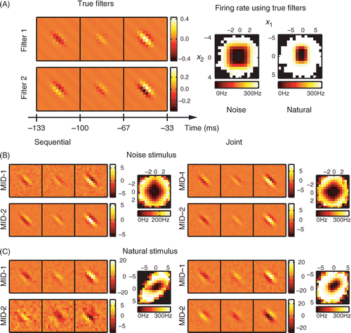
Figure 1. Joint optimization is required in the case of natural stimuli. (A) Spatiotemporal filters of the model neuron and associated nonlinear gain functions. Nonlinear gain functions were calculated from model responses to noise and natural stimuli. Axes of nonlinear gain functions are shown in units of standard deviation of the corresponding relevant dimensions. (B) Reconstruction in the case of noise stimuli. Optimization of one-dimensional information is sufficient to reconstruct the relevant dimensions of the model (subspace project O = 0.83±0.15). Joint optimization of two-dimensional information did not further improve the result (O = 0.8±0.2). (C) Natural stimulus. Joint optimization of relevant dimensions by maximizing the two-dimensional information markedly improves the subspace projection between model and reconstructed dimensions from 0.60 ± 0.04 to 0.875 ± 0.008. Note that the rotated nonlinear gain function in the relevant plane provides an equivalent description the system. Color-scale for each of the reconstructed filters represents signal-to-noise ratio.

Figure 2. Reconstruction of a model neuron with three relevant dimensions using joint search for three maximally informative dimensions (MID). (A) The three spatiotemporal filters of the model cell (left, each filter is normalized to length one, as in A) and associated nonlinear gain functions with respect to each of the relevant stimulus component considered individually (middle) or in pairs (right). Nonlinearities are calculated from model responses to natural stimuli. (B) Results of the reconstruction from responses to natural stimuli (the number of stimulus frames was ∼50 000). Optimization of joint information between spikes and three dimensions is able to recover all three dimensions of the model. The subspace projection between the model and reconstructed dimensions is O = 0.829 ± 0.005, cf. Equation (24). Notations are as in .
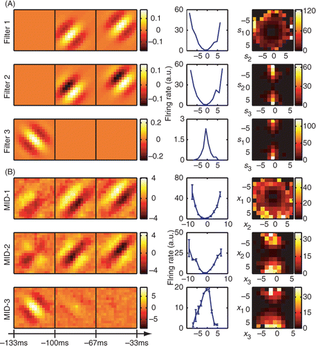
Figure 2. Reconstruction of a model neuron with three relevant dimensions using joint search for three maximally informative dimensions (MID). (A) The three spatiotemporal filters of the model cell (left, each filter is normalized to length one, as in Figure 1A) and associated nonlinear gain functions with respect to each of the relevant stimulus component considered individually (middle) or in pairs (right). Nonlinearities are calculated from model responses to natural stimuli. (B) Results of the reconstruction from responses to natural stimuli (the number of stimulus frames was ∼50 000). Optimization of joint information between spikes and three dimensions is able to recover all three dimensions of the model. The subspace projection between the model and reconstructed dimensions is O = 0.829 ± 0.005, cf. Equation (24). Notations are as in Figure 1.

Figure 3. Reconstruction of a model neuron with three relevant dimensions using projection pursuit regression (PPR). The three relevant dimensions of this model neuron are shown in and the nonlinear gain function is given by Equation (25). The reconstruction was done on the longer natural stimulus ensemble (∼50 000 frames). The subspace projection between the model and reconstructed dimensions is O = 0.59 ± 0.11, smaller than that obtained with the joint search for relevant dimensions using information maximization. Notations are as in .
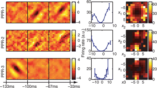
Figure 3. Reconstruction of a model neuron with three relevant dimensions using projection pursuit regression (PPR). The three relevant dimensions of this model neuron are shown in Figure 2 and the nonlinear gain function is given by Equation (25). The reconstruction was done on the longer natural stimulus ensemble (∼50 000 frames). The subspace projection between the model and reconstructed dimensions is O = 0.59 ± 0.11, smaller than that obtained with the joint search for relevant dimensions using information maximization. Notations are as in Figure 1.

Figure 4. Convergence of the joint and sequential information maximization with increasing number of spikes. Subspace projection, Equation (24), between the model and reconstructed dimensions (y-axis) is plotted as a function of the ratio of stimulus dimensionality (D) times the number of relevant dimensions (K) to the number of spikes (x-axis). Small x-values correspond to good sampling (high signal-to-noise ratio). Results for model cells with K equal to 1, 2, and 3 are shown in green, red, and blue, respectively. Results obtained with joint information maximization (circles) are always better than those obtained with sequential information maximization (squares). By construction, they are identical for 1D model cell. In the case of 3D model cell, sequential optimization did not converge to the true subspace with increasing number of spikes. Note that the number of spikes needed to achieve the same quality of reconstruction increases linearly with the number K of reconstructed dimensions.
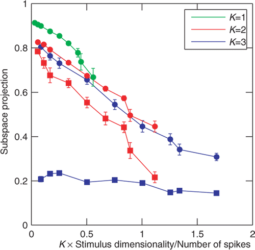
Figure 4. Convergence of the joint and sequential information maximization with increasing number of spikes. Subspace projection, Equation (24), between the model and reconstructed dimensions (y-axis) is plotted as a function of the ratio of stimulus dimensionality (D) times the number of relevant dimensions (K) to the number of spikes (x-axis). Small x-values correspond to good sampling (high signal-to-noise ratio). Results for model cells with K equal to 1, 2, and 3 are shown in green, red, and blue, respectively. Results obtained with joint information maximization (circles) are always better than those obtained with sequential information maximization (squares). By construction, they are identical for 1D model cell. In the case of 3D model cell, sequential optimization did not converge to the true subspace with increasing number of spikes. Note that the number of spikes needed to achieve the same quality of reconstruction increases linearly with the number K of reconstructed dimensions.

Figure 5. Reconstruction of an example V1 simple cell. (left) Two excitatory spatiotemporal filters (MID-1 and MID-2) and one inhibitory filter (MID-3). (right) The associated one- and two-dimensional non-linear firing rate functions are consistent with the properties of simple cells and nonlinear gain control model. Neuron 761 − 1.
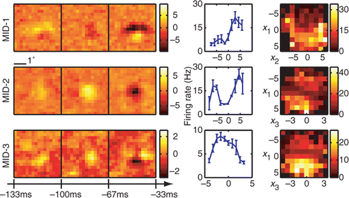
Figure 5. Reconstruction of an example V1 simple cell. (left) Two excitatory spatiotemporal filters (MID-1 and MID-2) and one inhibitory filter (MID-3). (right) The associated one- and two-dimensional non-linear firing rate functions are consistent with the properties of simple cells and nonlinear gain control model. Neuron 761 − 1.

Figure 6. Reconstruction of an example V1 complex cell. (left) Three-dimensional spatiotemporal receptive fields for a complex cell from V1. (right) The associated one- and two-dimensional nonlinear gain functions. Neuron 946 − 2. Notations are as in .
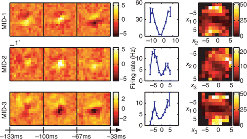
Figure 6. Reconstruction of an example V1 complex cell. (left) Three-dimensional spatiotemporal receptive fields for a complex cell from V1. (right) The associated one- and two-dimensional nonlinear gain functions. Neuron 946 − 2. Notations are as in Figure 1.

Figure 7. Comparison of joint and sequential methods on the responses of V1 neurons to natural stimuli. (A) Information about the responses of V1 neurons (n = 47) explained by three spatiotemporal dimensions estimated using either joint or sequential information maximization as a fraction of the total information per spike. Filled circles indicate cells where the joint information and sequential information were significantly different (p < 0.05). Overall, joint information maximization performed significantly better than sequential information maximization (p < 10−4, paired t-test). (B) Comparison between joint information maximization and projection pursuit regression. Joint information maximization performed significantly better than projection pursuit regression (p < 10−4, paired t-test). (C) Comparison between sequential information maximization and projection pursuit regression. The performance of the two methods was not significantly different (p = 0.75, paired t-test). All information values were evaluated using a set not used in estimations of the relevant dimensions.
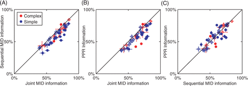
Figure 7. Comparison of joint and sequential methods on the responses of V1 neurons to natural stimuli. (A) Information about the responses of V1 neurons (n = 47) explained by three spatiotemporal dimensions estimated using either joint or sequential information maximization as a fraction of the total information per spike. Filled circles indicate cells where the joint information and sequential information were significantly different (p < 0.05). Overall, joint information maximization performed significantly better than sequential information maximization (p < 10−4, paired t-test). (B) Comparison between joint information maximization and projection pursuit regression. Joint information maximization performed significantly better than projection pursuit regression (p < 10−4, paired t-test). (C) Comparison between sequential information maximization and projection pursuit regression. The performance of the two methods was not significantly different (p = 0.75, paired t-test). All information values were evaluated using a set not used in estimations of the relevant dimensions.