A modal age at death approach to forecasting adult mortality

Abstract

Recent studies have shown that there are some advantages to forecasting mortality with indicators other than age-specific death rates. The mean, median, and modal ages at death can be directly estimated from the age-at-death distribution, as can information on lifespan variation. The modal age at death has been increasing linearly since the second half of the twentieth century, providing a strong basis from which to extrapolate past trends. The aim of this paper is to develop a forecasting model that is based on the regularity of the modal age at death and that can also account for changes in lifespan variation. We forecast mortality at ages 40 and above in 10 West European countries. The model we introduce increases forecast accuracy compared with other forecasting models and provides consistent trends in life expectancy and lifespan variation at age 40 over time.

Keywords:

• mortality
• forecast
• modal age at death
• lifespan variation
• life expectancy

Introduction

The rise in life expectancy over the last two centuries is one of the most remarkable achievements of human populations. Life expectancy at birth was around 40 years in the middle of the nineteenth century and reached 87 years for females in Japan in 2020 (Oeppen and Vaupel 2002; HMD 2022). This constant increase has led to important demographic and societal changes, such as population growth and ageing. Due to these continuing mortality changes and related consequences, public and private institutions rely on mortality forecasting to anticipate healthcare needs and pension costs, for example. The last few decades have witnessed an important increase in the number of forecasting models.

One model recurrently used for forecasting mortality is the Lee–Carter (LC) model (Lee and Carter 1992), which forecasts age-specific death rates log-bilinearly. The advantages of the LC model include its simplicity, the limited subjective judgement required, and its direct forecasts of the risk of death over time. However, the accuracy of this model is often questioned. The LC model assumes a constant rate of mortality improvement in age-specific death rates over time, but evidence shows that there has been accelerated mortality decline at older ages in some populations (Rau et al. 2008; Vaupel et al. 2021). Thus, the assumption often leads to the method under-predicting life expectancy (Lee and Miller 2001; Bergeron-Boucher and Kjærgaard 2022). Variants of the LC model have been suggested over the years, to improve the accuracy of the original model (Booth et al. 2002; Booth et al. 2006; Li and Lee 2005; Hyndman and Ullah 2007; Currie 2013; Li et al. 2013; Camarda and Basellini 2021).

Many forecasting models are based on the extrapolation of age-specific death rates, as these rates are indicative of the change in the risk of dying over time and, in addition, serve as the point of entry to the life table (Basellini and Camarda 2019). However, mortality forecasts can use a number of other meaningful demographic indicators as inputs (Bergeron-Boucher et al. 2019a). Some authors have suggested forecasting age-specific death probabilities (Cairns et al. 2006; King and Soneji 2011). Using either age-specific death rates or probabilities as inputs to the same model generally leads to similar forecasted trends (Bergeron-Boucher et al. 2019a). Other input indicators, such as life expectancy (Raftery et al. 2012; Torri and Vaupel 2012; Pascariu et al. 2018) and the age-at-death distribution (Oeppen 2008; Bergeron-Boucher et al. 2017; Basellini and Camarda 2019), have gained popularity, as they allow for changes in age-specific rates of mortality improvement (ASRMI).

Using life expectancy as the input has the advantage of directly forecasting the average duration of life, and it is the most popular measure of longevity. Life expectancy, as an aggregate indicator, is less volatile than age-specific measures of mortality. The associated forecasting models are not only more robust but also more parsimonious (Bergeron-Boucher et al. 2019a). However, life expectancy does not provide any information about age-specific mortality trends and levels, and researchers must rely on an additional model to derive age-specific mortality from the life expectancy values (Ševčíková et al. 2016; Pascariu et al. 2020; Nigri et al. 2022). As such, if information on death rates or probability of survival to certain ages (e.g. age at retirement) is needed, models based on life expectancy lose their parsimony.

The age-at-death distribution readily provides information on central longevity measures: the mean, median, and mode (Canudas-Romo 2010). While the mean (life expectancy) is the most used measure, the mode is increasingly seen as an alternative measure of longevity (Canudas-Romo 2008; Horiuchi et al. 2013). The modal age at death, M, is the age at which the most adult deaths occur. In low-mortality countries, M has been increasing since the 1930s–40s for females and since the 1970s for males (Canudas-Romo 2010; Bergeron-Boucher et al. 2015; Diaconu et al. 2016). An increase in the modal age at death indicates that the age-at-death distribution is shifting towards older ages, a dynamic interpreted as postponement of the mortality schedule. The latter, also referred to as shifting mortality, has been the dominant determinant of life expectancy increase in low-mortality countries since the middle of the twentieth century (Canudas-Romo 2008; Bongaarts 2009; Bergeron-Boucher et al. 2015). Increases in the modal age at death are driven primarily by decreases in mortality at older ages (Horiuchi et al. 2013; Diaconu et al. 2020), especially at ages above the mode (Canudas-Romo 2010), making this indicator particularly relevant for studying longevity extension.

Additionally, the age-at-death distribution provides information about the variability of lifetimes. This measure, also called lifespan variation, captures inequalities in lifespans from a population perspective. Lifespan variation can be directly calculated from the age-at-death distribution and is increasingly seen as a relevant complement to life expectancy and the modal age at death (Tuljapurkar 2001; Vaupel et al. 2011; van Raalte et al. 2018). Lifespan variation has been decreasing in most low-mortality populations since the late nineteenth century (Edwards and Tuljapurkar 2005), and this has led to a compression of mortality around the mode. Unlike shifting mortality, mortality compression (or reduction in lifespan variation) is driven by a reduction in mortality at younger ages (Aburto et al. 2020). There is, generally, a negative correlation between life expectancy and lifespan variation, as both measures are sensitive to mortality changes at younger ages. However, this is not a mechanical relationship, and many exceptions where lifespan variation increases with life expectancy have been documented (van Raalte et al. 2011; Brønnum-Hansen 2017; Aburto and van Raalte 2018; van Raalte et al. 2018).

The age-at-death distribution is increasingly used as an input to mortality forecasting models (Oeppen 2008; Bergeron-Boucher et al. 2017; Basellini and Camarda 2019; Aliverti et al. 2022; Shang et al. 2022). Basellini and Camarda (2019) introduced an innovative model to forecast the location (mode) and variability of the age-at-death distribution directly, based on a segmented transformation of the age-at-death distribution (STAD). The authors modelled and forecasted the differences between a standard and an observed distribution, using a transformation function that depends on the changes in these differences in the mode, differences in variability before the mode, and differences in variability after the mode. This model directly captures the two main mortality dynamics: shifting and compression of mortality. Oeppen (2008) also developed a forecasting model based on the age-at-death distribution. He used compositional data analysis (CoDA) to model and forecast a redistribution of deaths across age groups (usually from younger to older ages). Compositions are vectors containing positive values that represent parts of a whole and carry relative information summing up to a constant (e.g. proportions). CoDA is a set of tools that allows for the correct modelling of compositions, including distributions (Aitchison 1982). The use of the age-at-death distribution and CoDA in forecasting takes age dependency into account: due to the sum constraints, deaths in the life table are directly dependent on each other at the aggregate level, such that a decrease in deaths at one age will lead to an increase in deaths in at least one other age group. This property of the model resolves independence problems between mortality components in forecasting, including causes of death (Kjærgaard et al. 2019). The use of CoDA for forecasting mortality has attracted attention in recent years (Bergeron-Boucher et al. 2017; Kjærgaard et al. 2019; Kjærgaard et al. 2020; Shang et al. 2022).

In this paper, we aim to develop a new forecasting model that is based on the regularity of the modal age at death and that can also account for changes in lifespan variation. We use a CoDA approach to forecast the distribution centred around the modal age at death and forecast M independently. We call our model the Mode model. It captures both the shifting and compression of mortality, directly modelling the two main mortality dynamics as two distinct metrics.

The paper is organized as follows. In the Data section, we describe the data set used and the populations analysed. The Methods section starts with a description of a smoothing procedure, and we then describe how we estimate and forecast the modal age at death. We next introduce a CoDA model for forecasting the age-at-death distribution centred around the modal age at death; this model captures changes in lifespan variation. The remaining Methods subsections present how we calculate prediction intervals and how we estimate forecasting accuracy via an out-of-sample analysis, respectively. In the Results section, we provide an illustration of the methods by forecasting mortality for females and males in 10 West European countries. First, we present the parameters of the model and discuss their interpretation; second, we present the results of the out-of-sample analysis, comparing the proposed model with four other models; and, third, we show the forecasts up to 2050. Finally, in the Discussion, we review the methods and results, adding concluding remarks.

Data

We forecast mortality in 10 West European countries: Denmark, Finland, France, Ireland, the Netherlands, Norway, Portugal, Spain, Sweden, and Switzerland. This provides a mixture of countries with low, medium, and high mortality levels, as well as faster and slower rates of mortality progress. See Appendix A in the supplementary material for further information on the selection of countries. We use death counts and exposures from the Human Mortality Database (HMD 2022) from 1960 to 2019 (the last year with available data for all countries), for males and females aged 40–110 by single year of age.

Methods

We introduce a new forecasting model, labelled the Mode model, which is based on change in the modal age at death. The model consists of three main steps: (1) smoothing; (2) estimating and forecasting the modal age at death; (3) estimating and forecasting the age at death distribution centred around the mode.

Smoothing

Mortality is smoothed using a Poisson P-spline approach. We take the observed unsmoothed death counts and exposure from the HMD and smooth them using the R package MortalitySmooth (Camarda 2012). From these smoothed death rates, we calculate life tables. The smoothed age-at-death distribution is necessary for estimating the modal age at death, as described next.

Estimating and forecasting the modal age at death

The modal age at death (M) is the age at which the most deaths occur. The estimation of M is not straightforward, as the age-at-death distribution is not always smooth and random fluctuations can result in multiple maxima in the density of adult deaths. Several approaches to overcoming the irregular patterns of deaths around the mode have been suggested. Parametric models, such as the Gompertz or Siler models, have been used to smooth the mortality curve and calculate the mode (Canudas-Romo 2008). However, these models assume specific mortality shapes. Non-parametric approaches for estimating M have also been suggested, for example the Kannisto method (Kannisto 2001) and the P-spline approach (Ouellette and Bourbeau 2011). In this paper, we follow the method for estimating M suggested by Ouellette and Bourbeau (2011), where the age-at-death distribution is smoothed with a Poisson P-spline approach (Eilers and Marx 1996).

M has been increasing linearly since the middle of the twentieth century in most developed countries (Horiuchi et al. 2013). As a result of this linear development, we forecast M using a random walk with drift.

Estimating and forecasting the distribution around M

The forecast of the distribution around M requires three sub-steps: (1) recentring the age-at-death distribution around M; (2) forecasting the distribution with a CoDA model; and (3) completing the distribution for ages not supported by the forecasted distribution of deaths.

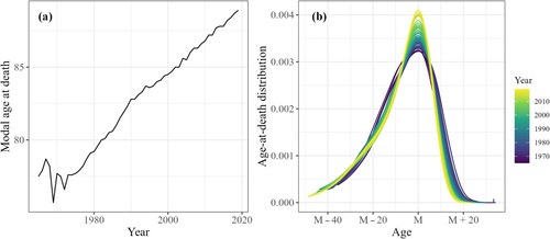
First, the age-at-death distribution around M can be expressed as a vector, $\mathit{d}=\left[d_{M-20},d_{M-19},\dots ,d_{M-1},d_M,d_{M+1},\dots ,d_{M+20}\right]$, with $d_x$ being the life-table deaths. This vector can be interpreted as an indicator of lifespan variation, that is, how compressed the lifespan distribution is around M. The $d_x$ centred around M are arranged in a matrix by time t and age x−M, which is notated D, where each row sums to unity and thus is compositional data. The location (M) and scale (D) of age-at-death distributions are then forecasted separately, that is, we model and forecast the shifting and compression of mortality as two separate metrics. Figure 1 illustrates changes in M and D over time for males in France. Figure 1(a) shows the linear development of M, and Figure 1(b) shows that deaths are increasingly concentrated around M over time.

Figure 1 (a) Modal age at death, M, and (b) age-at-death distribution around the mode, D: males in France, 1965–2019 Source: Authors’ analysis of data from HMD (2022).

Second, the smoothed age-at-death distribution around M can be forecasted using the CoDA approach (Oeppen 2008). In the case of mortality compression, the model forecasts a redistribution of deaths towards M and is defined as: (1) $\mathrm{clr}\left(d_{t,x-M}\ominus {\alpha }_{x-M}\right)={\kappa }_t{\text{β}}_{x-M}+{ϵ}_{t,x-M},$(1) where $d_{t,x-M}$ is the age-at-death distribution at time t and age x−M, and ${\alpha }_{x-M}$ is the age-specific average of $d_{t,x-M}$ over time. The clr is the centred log-ratio transformation, and $\ominus$ is a perturbation operator (Aitchison 1982). The parameter ${\kappa }_t$ is the time index, and ${\text{β}}_{x-M}$ is the age-specific sensitivity to ${\kappa }_t$. The latter indicates which ages gain deaths over time, relative to M, and which lose deaths in relative terms. The parameters ${\kappa }_t$ and ${\text{β}}_{x-M}$ are estimated from a generalized singular value decomposition (GSVD). The GSVD allows weights to be assigned to the age and time dimensions. We use a similar approach to that of Kjærgaard et al. (2019) to assign the weights. The age-specific weights are determined by the mean age-at-death distribution over time, thus giving more weight to the mode and the ages around it than to ages further from the mode. For the weights on the time dimension ($w_t$), we follow the approach of Hyndman et al. (2013), where more weight is given to the latest years observed than to earlier years: (2) $w_t=\rho (1-\rho {)}^{T-t},$(2) where $\rho$ determines the percentage weight for the most recent year (T). We use a $\rho$ of 5 per cent as suggested by Kjærgaard et al. (2019).

The time index parameter, ${\kappa }_t$, is not always linear. This feature is also observed when looking at measures of lifespan variation (Edwards and Tuljapurkar 2005; van Raalte et al. 2018). When forecasting non-linear trends, Hyndman and Athanasopoulos (2018) suggested using a natural cubic smoothing spline (which is a cubic spline with some constraints), so that the spline function is linear at the end (Hyndman et al. 2012). We use this approach to forecast ${\kappa }_t$.

Third, as M increases, the age range that supports the distribution of deaths in the forecast varies over time. More precisely, we obtain less and less information about the left tail of the distribution, that is, mortality at young ages. To remedy this problem, we assume that the missing values in the left tail of the distribution are equal to $d_{t,x+1}\times \widehat{R_x}$, where $\widehat{R_x}$ is the ratio of $d_{t,x}$ between two consecutive ages at the last year of observation: $\widehat{R_x}={\displaystyle \frac{d_{T,x}}{d_{T,x+1}}}$. We also tested extrapolating the left tail using the penalized composite link model for ungrouping (Rizzi et al. 2015) and a monotonic interpolating spline and find that the model based on ratios provides the most satisfactory results. As $d_{t,x}$ values are usually small at the beginning of the selected age interval, how we estimate the missing $d_{t,x}$ has only a minor impact on the forecast results.

Prediction intervals

Prediction intervals are estimated by a bootstrapping procedure based on fitting errors from both time-series models used to forecast M and ${\kappa }_t$. For each time series (M and ${\kappa }_t$), we compute 200 simulations. For each simulation of ${\kappa }_t$, we calculate the corresponding D. We then calculate age-at-death distributions for all possible combinations of simulated M and $\mathit{D}$, corresponding to 40,000 (200 × 200) simulated distributions. Relevant indicators (e.g. life expectancy and lifespan variation) are calculated for all simulations, and 95 per cent prediction intervals are calculated from the simulations by taking the 2.5th and 97.5th percentiles. We do not account for the errors induced by smoothing the age-at-death distribution when calculating the prediction intervals.

Out-of-sample approach

We use an out-of-sample approach based on different fitting periods and forecast horizons to evaluate forecasting accuracy. Forecasts are sensitive to both these components. We forecast mortality for each country starting from each year between 1994 and 2014 and forecasting up to 2019, representing forecast horizons varying from 25 to five years (21 forecasts). For each forecast horizon, the fitting period starts in either 1960, 1965, 1970, or 1975 (four forecasts) and thus its length varies from 55 to 20 years. As a result, we make 84 forecasts (21 × 4) for each country and sex.

We measure accuracy by the root mean square error, using different indicators: (1) life expectancy at age 40, $e_{40}$; (2) the modal age at death, M; (3) lifespan variation; and (4) logarithmic age-specific death rates,$\ln \left(m_x\right)$. Lifespan variation is measured by the average years of life lost at age 40, $e^{†}$ (Vaupel and Canudas-Romo 2003). The errors in the logged death rates are more important at younger ages relative to older ages, due to the higher logged values at younger ages. As such, mean errors in forecasting the age-specific logged death rates are driven by errors at younger ages, even if mortality at these ages is low. To remedy this problem, we weight the errors in logged death rates by the observed age-at-death distribution. Finally, the accuracy of the prediction intervals for life expectancy at age 40 is assessed by the percentage of observed values falling within the intervals.

We compare the accuracy of the Mode model with that of the LC model (Lee and Carter 1992), the functional data approach (FDA) (Hyndman and Ullah 2007; Hyndman et al. 2012), the CoDA model (Oeppen 2008), and the STAD model (Basellini and Camarda 2019). We select the LC model as this model has established itself as the standard and is one of the most used forecasting models (Basellini et al. 2023). We select the FDA as one possible variant of the LC model which generally improves its accuracy (Booth et al. 2006; Hyndman and Ullah 2007; Hyndman et al. 2012). The CoDA model is selected because our Mode model uses CoDA to forecast the variance around the mode and this comparison can show evidence of whether using the mode can improve the model, based on a similar method. Finally, the STAD model is selected as it is, to our knowledge, the only other model using the mode as an input to forecast period life expectancy. However, the modal age at death has been used as an input to forecast cohort mortality in the model of Rizzi et al. (2021). Predictions intervals for all selected models are based on a bootstrapping procedure on the time series, as suggested previously by Bergeron-Boucher et al. (2017) for the CoDA model and by Basellini and Camarda (2019) for the STAD model. The traditional LC model uses the innovation to calculate prediction intervals, which tends to lead to intervals that are too narrow. But methods using the bootstrap procedure have been suggested for the LC model, and these tend to lead to wider prediction intervals (Keilman and Pham 2006). A jump-off correction is carried out for all compared models, so that the observed and fitted values of the input (death rates or age-at-death distribution) at the jump-off year are the same. Correcting for the error at jump-off year improves accuracy for all models compared.

Results

Parameters

Figure 2 shows the estimated parameters M, ${\kappa }_t$, and ${\text{β}}_{x-M}$, and their forecasted values for males and females in France. M has been increasing linearly in France since the 1970s for males and since before the 1960s for females (Figure 2(a)). Similar results (not shown) are also found for the other nine countries, with the increase starting in the 1990s at the latest, for males in Denmark. Thus, a postponement in the mortality schedule has been seen in the last three to six decades across all countries and both sexes. Trends in the mode have generally been linear, which makes them easily extrapolatable by a linear model.

Figure 2 Observed and forecasted model parameters for the (a) modal age at death, M; (b) time index, ${\kappa }_t$; and (c) age pattern, ${\text{β}}_{x-M}$: males and females in France, 1965–2050

Source: As for Figure 1.

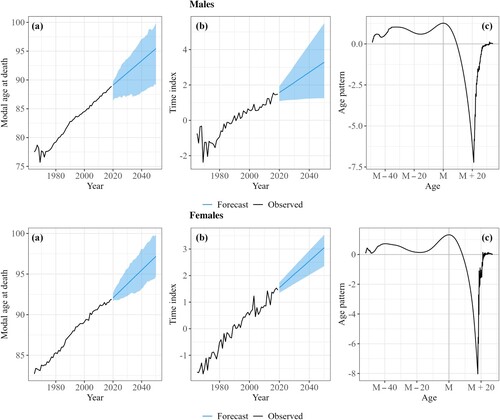
The parameters ${\kappa }_t$ and ${\text{β}}_{x-M}$ describe the change in the age-at-death distribution around M and capture how lifespan variation evolves over time. When ${\kappa }_t$ increases (Figure 2(b)), deaths are redistributed from ages with negative ${\text{β}}_{x-M}$ towards ages with positive ${\text{β}}_{x-M}$. Figure 2(c) shows that deaths have become increasingly redistributed towards M and the ages around it over time, capturing a compression of mortality around M. The ${\text{β}}_{x-M}$ profile is very similar across countries for males, but more variations are observed for females (see Appendix B, supplementary material). However, for all the selected countries and for both sexes, there has been a redistribution of deaths from ages about 10 years and more above the mode towards the modal age at death (highest value) and ages around it. This result indicates a compression of mortality around the increasing mode.

Out-of-sample analysis

Table 1 shows the mean forecasting errors in life expectancy at age 40 ($e_{40}$), the accuracy of the prediction intervals for $e_{40}$, and the mean forecasting errors in modal age at death (M), lifespan variation ($e^{†}$), and weighted logged age-specific death rates ($\ln \left(m_x\right)$) for five models: Mode, STAD, CoDA, FDA, and LC. Accuracy levels vary by sex, country, and model. However, on average, the Mode model is the most accurate in predicting $e_{40}$, M, and $\ln \left(m_x\right)$ for both males and females (see final column). As mortality postponement has been the main driver behind the increase in life expectancy since the middle of the twentieth century (Bergeron-Boucher et al. 2015), it should not be surprising that the model which can best predict M can also best predict life expectancy.

Table 1 Mean forecasting errors across 84 out-of-sample forecasts for life expectancy at age 40 (e₄₀), prediction interval accuracy for life expectancy at age 40, and mean forecasting errors in modal age at death (M), lifespan variation (e^†), and weighted logged death rates (In(m_x)), from the Mode, STAD, CoDA, FDA, and LC models: males and females in 10 West European countries

Males
	CHE	DNK	ESP	FIN	FRA	IRL	NLD	NOR	PRT	SWE	Mean (rank)
$e_{40}$
Mode	0.41	1.57	0.54	0.31	0.42	1.18	1.31	1.08	0.60	0.48	0.79 (1)
STAD	1.42	1.74	0.82	0.42	1.62	1.37	1.31	1.34	0.68	0.73	1.15 (4)
CoDA	0.75	1.74	0.52	0.54	0.45	1.98	1.68	1.44	1.24	0.96	1.13 (3)
FDA	0.92	1.59	1.62	0.59	1.00	1.46	1.80	1.11	1.28	1.05	1.24 (5)
LC	1.17	1.59	0.66	0.60	0.92	1.33	1.38	1.28	0.99	1.27	1.12 (2)
95 per cent prediction interval
Mode	99.2	93.3	99.9	100.0	98.8	98.0	68.6	83.8	99.9	99.0	87.3 (2)
STAD	52.9	55.1	69.9	96.6	56.9	69.1	60.0	57.2	80.0	84.6	68.2 (5)
CoDA	98.4	80.1	97.8	99.9	99.8	86.4	67.4	81.8	98.4	99.0	90.9 (1)
FDA	90.7	67.8	76.7	100.0	82.1	73.6	51.3	81.9	99.7	85.4	80.9 (3)
LC	89.2	39.2	94.7	93.8	96.1	64.7	60.9	49.9	94.7	88.3	77.1 (4)
M
Mode	0.42	2.23	0.71	0.79	0.34	1.96	1.77	1.43	0.90	0.61	1.12 (1)
STAD	1.53	2.93	1.17	1.12	1.59	2.56	2.03	1.95	1.32	1.11	1.73 (2)
CoDA	1.43	3.02	1.10	1.64	0.78	3.13	2.87	2.40	2.09	1.72	2.01 (4)
FDA	1.38	2.85	2.41	1.73	1.63	3.09	3.03	2.10	2.16	1.66	2.20 (5)
LC	1.73	2.80	1.22	1.76	1.51	2.86	2.45	2.07	1.65	1.84	1.99 (3)
$e^{†}$
Mode	0.19	0.17	0.29	0.29	0.23	0.18	0.12	0.19	0.11	0.10	0.19 (4)
STAD	0.38	0.37	0.51	0.36	0.39	0.17	0.11	0.16	0.18	0.16	0.28 (5)
CoDA	0.16	0.32	0.13	0.17	0.14	0.14	0.18	0.17	0.08	0.17	0.17 (2)
FDA	0.16	0.21	0.24	0.18	0.12	0.29	0.17	0.21	0.08	0.14	0.18 (3)
LC	0.19	0.21	0.15	0.22	0.10	0.22	0.08	0.12	0.08	0.19	0.16 (1)
$\ln \left(m_x\right)$
Mode	0.86	1.86	0.82	1.07	0.78	1.75	1.66	1.60	0.98	0.84	1.22 (1)
STAD	2.08	2.15	1.30	1.52	2.02	2.34	1.85	1.85	1.29	1.27	1.77 (5)
CoDA	1.05	1.78	0.78	1.09	0.75	2.27	1.73	1.66	1.46	1.15	1.37 (2)
FDA	1.24	1.85	1.65	1.24	1.13	2.19	1.88	1.62	1.55	1.25	1.56 (4)
LC	1.53	1.82	0.97	1.36	1.14	2.14	1.61	1.72	1.42	1.46	1.52 (3)
Females
	CHE	DNK	ESP	FIN	FRA	IRL	NLD	NOR	PRT	SWE	Mean (rank)
$e_{40}$
Mode	0.53	1.06	0.50	0.40	0.60	0.65	0.37	0.36	0.50	0.29	0.53 (1)
STAD	0.43	1.30	0.78	0.40	0.65	1.49	0.42	1.40	1.22	0.19	0.83 (5)
CoDA	1.11	1.34	0.45	0.68	0.85	1.22	0.53	0.71	1.03	0.28	0.82 (4)
FDA	0.31	1.44	0.38	0.29	0.39	1.02	0.65	1.03	0.56	0.17	0.62 (2)
LC	1.21	1.38	0.33	0.31	0.41	0.89	0.54	0.57	1.67	0.20	0.75 (3)
95 per cent prediction interval
Mode	99.0	91.5	95.2	100.0	92.9	99.8	99.8	100.0	100.0	99.7	97.8 (2)
STAD	99.9	65.0	96.5	99.8	99.3	92.8	91.6	48.1	93.3	99.7	88.6 (5)
CoDA	98.9	99.4	100.0	100.0	100.0	100.0	100.0	100.0	100.0	100.0	99.8 (4)
FDA	98.8	79.4	100.0	100.0	98.2	83.1	93.8	97.8	99.8	100.0	95.1 (1)
LC	98.2	62.2	99.3	99.9	96.5	78.4	93.7	99.3	93.3	100.0	92.1 (3)
M
Mode	0.68	0.50	0.52	0.45	0.52	1.01	0.38	0.22	0.51	0.44	0.52 (1)
STAD	0.46	0.86	0.77	0.46	0.38	2.32	0.54	1.61	1.02	0.36	0.88 (5)
CoDA	0.98	0.81	0.34	0.54	0.39	1.65	0.53	0.78	1.08	0.22	0.73 (4)
FDA	0.25	0.78	0.45	0.47	0.41	1.14	0.64	1.02	0.57	0.19	0.59 (2)
LC	1.05	0.71	0.38	0.42	0.32	1.12	0.49	0.54	1.48	0.21	0.67 (3)
$e^{†}$
Mode	0.27	0.50	0.10	0.15	0.09	0.15	0.22	0.19	0.22	0.15	0.20 (3)
STAD	0.18	0.57	0.16	0.15	0.13	0.11	0.28	0.29	0.23	0.21	0.23 (4)
CoDA	0.27	0.51	0.33	0.19	0.33	0.16	0.15	0.17	0.17	0.08	0.24 (5)
FDA	0.10	0.54	0.18	0.13	0.15	0.12	0.19	0.22	0.10	0.08	0.18 (1)
LC	0.25	0.45	0.21	0.15	0.15	0.12	0.13	0.12	0.21	0.08	0.19 (2)
$\ln \left(m_x\right)$
Mode	1.08	1.31	0.82	1.04	0.87	1.24	0.75	0.91	0.93	0.74	0.96 (1)
STAD	1.16	1.59	1.10	1.41	0.92	2.34	0.94	2.09	1.73	0.88	1.42 (5)
CoDA	1.37	1.46	0.88	1.20	1.10	1.64	0.80	1.09	1.31	0.68	1.15 (3)
FDA	0.91	1.59	0.86	1.16	0.78	1.65	0.96	1.48	1.00	0.73	1.11 (2)
LC	1.48	1.59	0.85	1.30	0.79	1.69	0.92	1.23	1.92	0.82	1.26 (4)

Note: Values in bold indicate the model providing the most accurate forecasts. Mean forecasting errors are across the 84 out-of-sample forecasts for each country. The final column shows the mean errors across all countries combined.

Source: Authors’ analysis of data from HMD (2022).

Bohk-Ewald et al. (2017) have noted that the evaluation of forecasting models based on life expectancy alone is not sufficient, as such an evaluation cannot determine whether or not the underlying mortality developments are plausible. They suggest also evaluating whether lifespan variation forecasts are plausible, to check that forecasts can accurately predict the mortality scale. As shown in Table 1, forecasting errors for $e^{†}$ are generally smaller than those for M and $e_{40}$ for all selected models. As a result, the accuracy of the models is not undermined by looking at this indicator. Although the STAD model’s forecast accuracy is fair in predicting M (for males), it provides a relatively low accuracy for $e^{†}$. The Mode model is more accurate than the STAD model in forecasting $e^{†}$, but the LC and FDA models are the models which provide, on average, the best accuracy for lifespan variation.

The CoDA model provides the most accurate prediction intervals for males, with 90.9 per cent of the observed life expectancy values falling within the prediction’s bands, on average. For females, the FDA model shows the most accurate prediction intervals, on average, with 95.1 per cent of the observed values falling within the interval. Using the Mode model yields 87.3 and 97.8 per cent accuracy for males and females, respectively.

The Mode model is the most accurate in forecasting age-specific death rates for both sexes, followed by the CoDA model for males and the FDA model for females. The CoDA model forecasts an increase in the ASRMI over time (Bergeron-Boucher et al. 2017), capturing more accurately, compared with other models, the recent accelerating decline in mortality at older ages for males and, to some extent, for females (ranked third for females). In Appendix C, supplementary material, we show that the ASRMI at older ages also increase with the Mode model, but eventually level off, unlike in the CoDA model.

Forecasts

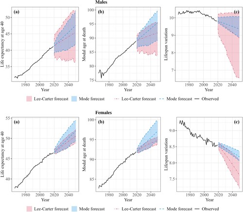
Figure 3 shows the life expectancy at age 40, modal age at death, and lifespan variation, observed from 1965 to 2019 and forecasted up to 2050 with the Mode and LC models, for males and females in France. The Mode model forecasts that life expectancy at age 40 in France will increase from 41.2 years in 2019 (between 38.9 and 42.9 years for the other countries) to 47.6 years (44.9–49.3 for the other countries) in 2050 for males and from 46.5 (44.1–46.8) years to 51.8 (48.4–51.9) years for females (Figure 3(a)). In comparison, the LC model forecasts an increase to 45.5 years (between 43.6 and 47.7 years for the other countries) by 2050 for males and 50.5 (46.2–51.0) for females. Compared with the LC model, the Mode model forecasts a faster increase in life expectancy and modal age at death (Figure 3(a–b)) but a slower decrease in lifespan variation (Figure 3(c)). The LC model tends to produce a change in the trends at the jump-off year, particularly for the modal age at death. The LC generally assumes that future gains in life expectancy will result from faster compression but slower postponement than gains in the past. As the increase in the mode is due mainly to mortality reduction above it, this result might come from the low and constant ASRMI at older ages assumed by the LC model. Meanwhile, the Mode model allows for increasing ASRMI at older ages. The model generally produces increasing ASRMI above age 85, constant or decreasing ASRMI between ages 65 and 85, and mixed trends below age 65, depending on the country and sex (see Appendix C, supplementary material).

Figure 3 (a) Life expectancy at age 40, $e_{40}$; (b) modal age at death, M; and (c) lifespan variation, $e^{†}$, observed and forecasted with the Mode and Lee–Carter models: males and females in France, 1965–2050

Note: The shaded areas represent the 95 per cent prediction intervals.

Source: As for Figure 1.

The forecasts using the Mode model generally continue past trends in $e_{40}$, M, and $e^{†}$, without noticeable trend breaks. Figure 4(a) shows that the forecasted trends in life expectancy at age 40 stay somewhat consistent for individual countries, but a divergence in trends is forecast between countries, with an increase in the range of life expectancy from 3.0 years in 2019 to 4.4 years in 2050 for males and from 2.7 to 3.5 years for females.

Figure 4 (a) Life expectancy at age 40, $e_{40}$; (b) modal age at death, M; and (c) lifespan variation, $e^{†}$, observed and forecasted with the Mode model: males and females in 10 West European countries, 1965–2050

Note: This figure is best viewed online in colour.

Source: As for Figure 1.

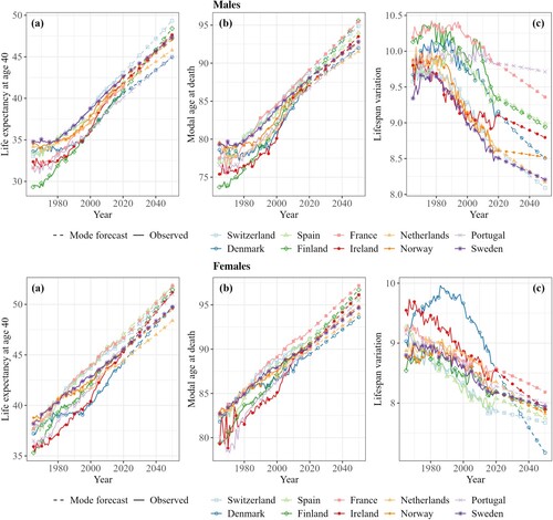
For females, M looks similar across all countries, except for Finland, Ireland, and Portugal, until the early 1990s. After then, the trends started to diverge, with slower improvements for Denmark, the Netherlands, and Sweden, where M reached lower levels similar to those in Finland, Ireland, and Portugal. The forecasts show persisting future divergence. For the Netherlands and Sweden, trends in $e_{40}$ and M are consistent, which might indicate that mortality at older ages in these countries is not decreasing as rapidly as in other countries. For females in Denmark, although $e_{40}$ stagnated between 1975 and 1995, we do not observe such great stagnation in M, despite slower improvement after 1990. This result hints that the $e_{40}$ stagnation for Denmark resulted from mortality worsening below the mode, as shown by the increase in $e^{†}$ (Figure 4(c)) and by other studies (Christensen et al. 2010; Lindahl-Jacobsen et al. 2016).

For males, the divergence in $e_{40}$ and M can be explained by the use of 1965–2019 as the fitting period for all countries. The mode started to increase only in the 1980s for males in the Netherlands and Sweden and in the 1990s for males in Denmark, but it has been increasing since 1970 for France, Switzerland, and Portugal. The forecasted increases in M may thus be slowed down by fitting the model over a period of stagnation, an issue most important in Denmark, the Netherlands, and Sweden.

Some divergence is also forecast in lifespan variation, mainly due to the influence of males in Portugal and females in Denmark (Figure 4(c)). The range of values of $e^{†}$ increases from 1.3 years in 2019 to 1.6 years in 2050 (1.3 without Portugal) for males and from 0.8 to 1.0 years for females (0.5 without Denmark). Since the 1990s there has been a small improvement in $e^{†}$ for males in Portugal and a rapid decrease for females in Denmark. The Mode model continues these trends in the forecast, which leads to a divergence in trends for females in Denmark and males in Portugal relative to their counterparts in other countries.

Discussion

The age-at-death distribution provides important information about mortality patterns and changes, longevity (postponement), and lifespan variation (compression). In addition, forecasting with the age-at-death distribution solves the dependency problems between components (with the use of specific models) and provides less biased forecasts than similar models based on death rates (Bergeron-Boucher et al. 2017; Kjærgaard et al. 2019). Yet, age-at-death distributions are not commonly used as inputs for forecasting models, especially compared with age-specific death rates or probabilities.

In this paper, we developed a model that builds on at least three major advantages that result from considering the age-at-death distribution as an input: the Mode model (1) uses the important regularity of an almost linear change in the modal age at death; (2) accounts for changes in lifespan variation; and also (3) considers the dependence between ages due to its use of the CoDA model. Our analysis revealed that the Mode model could, on average, better predict both the modal age at death and life expectancy at age 40 in 10 West European countries and for both sexes, compared with the other models considered. It also provides more accurate forecasts of the age-specific death rates and plausible trends in lifespan variation.

The modal age at death has increased linearly since the second half of the twentieth century in many low-mortality populations (Horiuchi et al. 2013), providing a strong basis from which to extrapolate past trends. In contrast to life expectancy, the modal age at death is not sensitive to potential increases or slowdowns in mortality at ages below it (Canudas-Romo 2010). A stagnation or decrease in life expectancy has been observed over some periods of time in different countries, including Denmark and the United States (US). It is often caused by mortality worsening at young- or mid-adult ages (Lindahl-Jacobsen et al. 2016; Woolf and Schoomaker 2019). For example, in Denmark, life expectancy stagnated for females between 1975 and 1995, due mainly to limited mortality improvement at mid-adult ages and a considerable burden from cancer mortality in specific birth cohorts (Christensen et al. 2010; Bergeron-Boucher et al. 2019b). However, no such stagnation was observed at older ages and, as a result, the modal age at death has been increasing in Denmark since the 1960s (or earlier) for females and the 1990s for males. Models that take advantage of this regular behaviour of the modal age at death can produce more accurate mortality forecasts for this country. The modal age at death is usually better suited than life expectancy to capturing the location of the age-at-death distribution, the speed of its shifting, and the increase in longevity.

Measures of central tendency, such as the mode or mean, are not sufficient to determine whether mortality forecasts are plausible, as similar values of the mode or mean can result from different mortality developments (Bohk-Ewald et al. 2017). Lifespan variation provides useful information about mortality scales and inequalities. A reduction in lifespan variation is observed in most populations, with deaths becoming increasingly compressed around the modal age at death (Kannisto 2001). The Mode model directly models and forecasts this dynamic, with the ${\text{β}}_{x-M}$ parameter capturing this redistribution of deaths towards the mode. Our results showed that the model can provide plausible trends in lifespan variation and good forecasting accuracy.

Another advantage of the Mode model is that its ASRMI can change over time, increasing at some ages and decreasing at others. Evidence shows that in low-mortality countries, mortality decline has been decelerating at younger ages but accelerating at older ages (Rau et al. 2008; Li et al. 2013; Vaupel et al. 2021). This pattern is referred to as a rotation (Li et al. 2013), which the Mode model is able to capture. The Mode and CoDA models allow for increasing ASRMI at older ages and generally produce more accurate forecasts of old-age mortality. At younger ages, the ASRMI tend to stagnate or slow down. The Mode model is also able to account for this dynamic. For ages below the mode, assuming constant or decreasing ASRMI (as implicit in the Mode and LC models) leads to better forecasts of the age-specific death rates.

Like other extrapolative models, the Mode model is sensitive to the fitting period selected. How to find the most relevant fitting period remains an open question. Generally, a longer fitting period will provide more accurate forecasts, but it is also important to select a fitting period that reflects an ongoing or emerging dynamic (Janssen and Kunst 2007; Bergeron-Boucher et al. 2019b). The year when M started to increase—a way of capturing the mortality postponement dynamic—differed by country and sex. The use of the same fitting period across all studied populations, for consistency, affected the accuracy of the forecasts. For males, using a more recent fitting period might have been more suitable.

Our proposed model is heavier in terms of its number of steps than other models, such as the LC model that directly forecasts age-specific mortality rates. Simplicity can help a model to be more widely used and is often cited as one of the main advantages of the LC model (Basellini et al. 2023). But sacrificing some simplicity can be justified if forecast accuracy can be significantly improved. The literature shows multiple examples of reasonable multistep approaches in forecasting. For example, the STAD model forecasts the compression and shifting dynamics independently. The United Nations (UN) forecasts life expectancy and then derives age-specific mortality patterns with a separate model (Raftery et al. 2012). Coherent forecasting models usually forecast a standard independently and forecast the population-specific deviation from this average as two separate steps; this generally improves the forecasts (Li and Lee 2005; Booth 2020).

Due to the Covid-19 pandemic, life expectancy declined in most countries in 2020 and 2021 (Aburto et al. 2022). Extrapolative models, such as those tested in this paper, cannot account for mortality shocks. As the last year observed for all selected countries in the HMD was 2019, the predicted life expectancies for 2020 and 2021, and potentially 2022, will most likely be too high. Previous mortality shocks, such as the Spanish flu and the two world wars, led to a decrease in life expectancy for a short period of time, after which life expectancy returned to its prior level within one or two years (Schöley et al. 2022). In this context, the models tested should still be relevant to forecasting post-pandemic mortality. However, whether or when mortality will return to its expected trajectory is still unclear.

The Mode model is limited to forecasting adult mortality patterns. Due to the shape of the human mortality pattern, using the full age range will create some fitting problems. For example, there is a second mortality peak at birth. When estimating the age-at-death distribution centred around M, the peak of infant deaths will be allocated to ages further and further away from M over time, creating an artificially fast mortality decline at the relative ages where the peak used to be. A similar issue will arise if we consider the ages at which the accident mortality hump appears (around ages 20–30). For this reason, we suggest limiting the forecast to mortality at ages 40 and above.

The proposed model has not been tested in cases where lifespan variation increases, such as the US since the 2010s (Acciai and Firebaugh 2019). It is unclear how the model will perform in such a context: this will depend on the ${\text{β}}_{x-M}$ pattern. If ${\text{β}}_{x-M}$ captures a redistribution of deaths towards ages below the mode, we might forecast an indefinite increase in lifespan variation. In such a context, an extension of the model could be developed to allow for changes (rotations) in ${\text{β}}_{x-M}$ over time, as previously suggested for the LC model (Li et al. 2013).

The Mode model can also be extended to reflect other mortality processes. For example, a coherent version of the model could be developed to account for non-diverging trends between countries or sexes, by forecasting the differences between the modal age at death and a reference trend. The changes in lifespan variation between countries could also be forecast by applying the coherent CoDA model from Bergeron-Boucher et al. (2017). Cause-of-death information or smoking-related mortality data could also be included in the model (Janssen et al. 2013; Kjærgaard et al. 2019). The use of CoDA makes the Mode model particularly adept at forecasting mortality by cause, due to its component-dependence modelling. We forecasted the modal age at death and the time index of the age-at-death distribution centred around the mode as two separate trends because, sometimes, they behave inconsistently. However, the two measures are very often negatively correlated and, in such cases, both indicators can be forecasted dependently. Kjærgaard et al. (2019) suggested using a cointegrated vector error model to account for dependence between multiple time indexes. It was, however, outside the scope of this paper to test all possible extensions of the proposed model.

Our model captures the two main mortality dynamics at adult ages: compression and shifting. These components are also well captured by the STAD model. The main difference between the two models is that the STAD model forecasts the difference between a standard age-at-death distribution and the observed distribution, whereas the Mode model directly forecasts the observed age-at-death distribution. The STAD model also forecasts three sets of parameters (the mode and the variation before and after the mode), whereas the Mode model forecasts two sets of parameters (M and ${\kappa }_t$).

We believe that the modal age at death is a solid basis for forecasting mortality, as this indicator has been increasing with few or no breaks in many populations since the second half of the twentieth century. This regularity, combined with M capturing mortality postponement and being easily combined with measures of scale and inequalities, makes the use of the modal age at death appealing for forecasting mortality. The Mode model we have introduced provides several advantages and can improve forecasting accuracy compared with other models. This is, however, only a first step, and potential extensions of the model (e.g. its coherent extension) should help to improve accuracy even more.

Disclosure statement

No potential conflict of interest was reported by the authors.

Notes

1 Please direct all correspondence to Marie-Pier Bergeron-Boucher, Interdisciplinary Centre on Population Dynamics, University of Southern Denmark, Campusvej 55, Odense 5230, Denmark; or by E-mail: [email protected].

2 Acknowledgement: This paper is dedicated to Jim W. Vaupel. He wanted to develop better forecasting models based on strong regularities in mortality trends and asked us to investigate how to forecast using the modal age at death. We are deeply thankful for his creativity and inspiring discussion. We also want to thank Silvia Rizzi for her help with ungrouping techniques.

3 Funding: The research leading to this publication is a part of a project that has received funding from the ROCKWOOL Foundation, through the research project ‘Challenges to the Implementation of Indexation of the Pension Age in Denmark’; from the European Research Council (ERC) under the European Union’s Horizon 2020 research and innovation programme (grant agreement number 884328—Unequal Lifespans); and by the AXA Research Fund, through the funding for the AXA Chair in Longevity Research.

References

- Aburto, José Manuel and Alyson van Raalte. 2018. Lifespan dispersion in times of life expectancy fluctuation: The case of Central and Eastern Europe, Demography 55(6): 2071–2096. https://doi.org/10.1007/s13524-018-0729-9
- Aburto, José Manuel, Jonas Schöley, Ilya Kashnitsky, Luyin Zhang, Charles Rahal, Trifon I. Missov, Melinda C. Mills, et al. 2022. Quantifying impacts of the COVID-19 pandemic through life-expectancy losses: A population-level study of 29 countries, International Journal of Epidemiology 51(1): 63–74. https://doi.org/10.1093/ije/dyab207
- Aburto, José Manuel, Francisco Villavicencio, Ugofilippo Basellini, Søren Kjærgaard, and James W. Vaupel. 2020. Dynamics of life expectancy and life span equality, Proceedings of the National Academy of Sciences 117(10): 5250–5259. https://doi.org/10.1073/pnas.1915884117
- Acciai, Francesco and Glenn Firebaugh. 2019. Twin consequences of rising U.S. death rates among young adults: Lower life expectancy and greater lifespan variability, Preventive Medicine 127: 105793. https://doi.org/10.1016/j.ypmed.2019.105793
- Aitchison, John. 1982. The statistical analysis of compositional data, Journal of the Royal Statistical Society: Series B (Methodological) 44(2): 139–160. https://doi.org/10.1111/j.2517-6161.1982.tb01195.x
- Aliverti, Emanuele, Stefano Mazzuco, and Bruno Scarpa. 2022. Dynamic modelling of mortality via mixtures of skewed distribution functions, Journal of the Royal Statistical Society Series A: Statistics in Society 185(3): 1030–1048. https://doi.org/10.1111/rssa.12808
- Basellini, Ugofilippo and Carlo Giovanni Camarda. 2019. Modelling and forecasting adult age-at-death distributions, Population Studies 73(1): 119–138. https://doi.org/10.1080/00324728.2018.1545918
- Basellini, Ugofilippo, Carlo Giovanni Camarda, and Heather Booth. 2023. Thirty years on: A review of the Lee–Carter method for forecasting mortality, International Journal of Forecasting 39(3): 1033–1049. https://doi.org/10.1016/j.ijforecast.2022.11.002
- Bergeron-Boucher, Marie-Pier, Vladimir Canudas-Romo, James Oeppen, and James W. Vaupel. 2017. Coherent forecasts of mortality with compositional data analysis, Demographic Research 37: 527–566. https://doi.org/10.4054/DemRes.2017.37.17
- Bergeron-Boucher, Marie-Pier, Marcus Ebeling, and Vladimir Canudas-Romo. 2015. Decomposing changes in life expectancy: Compression versus shifting mortality, Demographic Research 33: 391–424. https://doi.org/10.4054/DemRes.2015.33.14
- Bergeron-Boucher, Marie-Pier, and Søren Kjærgaard. 2022. Mortality forecasting at age 65 and above: An age-specific evaluation of the Lee-Carter model, Scandinavian Actuarial Journal 2022(1): 64–79. https://doi.org/10.1080/03461238.2021.1928542
- Bergeron-Boucher, Marie-Pier, Søren Kjærgaard, James Oeppen, and James W. Vaupel. 2019a. The impact of the choice of life table statistics when forecasting mortality, Demographic Research 41: 1235–1268. https://doi.org/10.4054/DemRes.2019.41.43
- Bergeron-Boucher, Marie-Pier, Søren Kjærgaard, Marius D. Pascariu, José Manuel Aburto, Ugofilippo Basellini, Silvia Rizzi, and James W. Vaupel. 2019b. Alternative forecasts of Danish life expectancy, in Stefano Mazzuco and Nico Keilman (eds), Developments in Demographic Forecasting. Cham: Springer, pp. 131–151.
- Bohk-Ewald, Christina, Marcus Ebeling, and Roland Rau. 2017. Lifespan disparity as an additional indicator for evaluating mortality forecasts, Demography 54(4): 1559–1577. https://doi.org/10.1007/s13524-017-0584-0
- Bongaarts, John. 2009. Trends in senescent life expectancy, Population Studies 63(3): 203–213. https://doi.org/10.1080/00324720903165456
- Booth, Heather. 2020. Coherent mortality forecasting with standards: Low mortality serves as a guide, in Stefano Mazzuco and Nico Keilman (eds), Developments in Demographic Forecasting. Cham, Switzerland: Springer, pp. 153–178.
- Booth, Heather, R. J. Hyndman, Leonie Tickle, and Piet de Jong. 2006. Lee-Carter mortality forecasting: A multi-country comparison of variants and extensions, Demographic Research 15: 289–310. https://doi.org/10.4054/DemRes.2006.15.9
- Booth, Heather, John Maindonald, and Len Smith. 2002. Applying Lee-Carter under conditions of variable mortality decline, Population Studies 56(3): 325–336. https://doi.org/10.1080/00324720215935
- Brønnum-Hansen, Henrik. 2017. Socially disparate trends in lifespan variation: A trend study on income and mortality based on nationwide Danish register data, BMJ Open 7(5): e014489.
- Cairns, Andrew, J. G. David Blake, and Kevin Dowd. 2006. A two-factor model for stochastic mortality with parameter uncertainty: Theory and calibration, Journal of Risk and Insurance 73(4): 687–718. https://doi.org/10.1111/j.1539-6975.2006.00195.x
- Camarda, Carlo Giovanni. 2012. Mortalitysmooth: An R package for smoothing Poisson counts with P-splines, Journal of Statistical Software 50: 1–24.
- Camarda, Carlo Giovanni and Ugofilippo Basellini. 2021. Smoothing, decomposing and forecasting mortality rates, European Journal of Population 37: 569–602. https://doi.org/10.1007/s10680-021-09582-4
- Canudas-Romo, Vladimir. 2008. The modal age at death and the shifting mortality hypothesis, Demographic Research 19: 1179–1204. https://doi.org/10.4054/DemRes.2008.19.30
- Canudas-Romo, Vladimir. 2010. Three measures of longevity: Time trends and record values, Demography 47(2): 299–312. https://doi.org/10.1353/dem.0.0098
- Christensen, Kaare, Michael Davidsen, Knud Juel, Laust Hvas Mortensen, Roland Rau, and James W. Vaupel. 2010. The divergent life-expectancy trends in Denmark and Sweden and some potential explanations, in E.M. Crimmins, Samuel Preston and Barney Cohen (eds), International Differences in Mortality at Older Ages: Dimensions and Sources. Washington, DC: The National Academies Press, pp. 385–407.
- Currie, Iain D. 2013. Smoothing constrained generalized linear models with an application to the Lee-Carter model, Statistical Modelling 13(1): 69–93. https://doi.org/10.1177/1471082X12471373
- Diaconu, Viorela, Nadine Ouellette, and Robert Bourbeau. 2020. Modal lifespan and disparity at older ages by leading causes of death: A Canada-U.S. comparison, Journal of Population Research 37(4): 323–344. https://doi.org/10.1007/s12546-020-09247-9
- Diaconu, Viorela, Nadine Ouellette, Carlo Giovanni Camarda, and Robert Bourbeau. 2016. Insight on ‘typical’ longevity: An analysis of the modal lifespan by leading causes of death in Canada, Demographic Research 35: 471–504. https://doi.org/10.4054/DemRes.2016.35.17
- Edwards, Ryan D. and Shripad Tuljapurkar. 2005. Inequality in life spans and a new perspective on mortality convergence across industrialized countries, Population and Development Review 31(4): 645–674. https://doi.org/10.1111/j.1728-4457.2005.00092.x
- Eilers, Paul H. C. and Brian D. Marx. 1996. Flexible smoothing with B-splines and penalties, Statistical Science 11(2): 89–102.
- HMD. 2022. Human Mortality Database. University of California, Berkeley (USA), and Max Planck Institute for Demographic Research (Germany), Accessed on 6 September. www.mortality.org.
- Horiuchi, Shiro, Nadine Ouellette, Karen S. L. Cheung, and Jean-Marie Robine. 2013. Modal age at death: Lifespan indicator in the era of longevity extension, Vienna Yearbook of Population Research 11: 37–69. https://doi.org/10.1553/populationyearbook2013s37
- Hyndman, Rob J. and George Athanasopoulos. 2018. Forecasting: Principles and Practice. Melbourne, Australia: OTexts.
- Hyndman, Rob J. and Md Shahid Ullah. 2007. Robust forecasting of mortality and fertility rates: A functional data approach, Computational Statistics & Data Analysis 51(10): 4942–4956. https://doi.org/10.1016/j.csda.2006.07.028
- Hyndman, R. J., H. Booth, and F. Yasmeen. 2013. Coherent mortality forecasting: The product-ratio method with functional time series models, Demography 50(1): 261–283. https://doi.org/10.1007/s13524-012-0145-5
- Hyndman, Rob J., Heather Booth, Leonie Tickle, and John Maindonald. 2012. Demography: Forecasting mortality, fertility, migration and population data. R package version 1.16.
- Janssen, Fanny and Anton Kunst. 2007. The choice among past trends as a basis for the prediction of future trends in old-age mortality, Population Studies 61(3): 315–326. https://doi.org/10.1080/00324720701571632
- Janssen, Fanny, Leo J. van Wissen, and Anton E. Kunst. 2013. Including the smoking epidemic in internationally coherent mortality projections, Demography 50(4): 1341–1362. https://doi.org/10.1007/s13524-012-0185-x
- Kannisto, Vaino. 2001. Mode and dispersion of the length of life, Population: An English Selection 13(1): 159–171.
- Keilman, Nico and Dinh Quang Pham. 2006. “Prediction intervals for Lee-Carter-based mortality forecasts.” European Population Conference, Liverpool.
- King, Gary and Samir Soneji. 2011. The future of death in America, Demographic Research 25: 1–38. https://doi.org/10.4054/DemRes.2011.25.1
- Kjærgaard, Søren, Yunus Emre Ergemen, Marie-Pier Bergeron-Boucher, Jim Oeppen, and Malene Kallestrup-Lamb. 2020. Longevity forecasting by socio-economic groups using compositional data analysis, Journal of the Royal Statistical Society Series A: Statistics in Society 183(3): 1167–1187. https://doi.org/10.1111/rssa.12555
- Kjærgaard, Søren, Yunus Emre Ergemen, Malene Kallestrup-Lamb, Jim Oeppen, and Rune Lindahl-Jacobsen. 2019. Forecasting causes of death by using compositional data analysis: The case of cancer deaths, Journal of the Royal Statistical Society Series C: Applied Statistics 68(5): 1351–1370. https://doi.org/10.1111/rssc.12357
- Lee, Ronald D. and Lawrence R. Carter. 1992. Modeling and forecasting US mortality, Journal of the American Statistical Association 87(419): 659–671.
- Lee, Ronald and Timothy Miller. 2001. Evaluating the performance of the Lee-Carter method for forecasting mortality, Demography 38(4): 537–549. https://doi.org/10.1353/dem.2001.0036
- Li, Nan and Ronald Lee. 2005. Coherent mortality forecasts for a group of populations: An extension of the Lee-Carter method, Demography 42(3): 575–594. https://doi.org/10.1353/dem.2005.0021
- Li, Nan, Ronald Lee, and Patrick Gerland. 2013. Extending the Lee-Carter method to model the rotation of age patterns of mortality decline for long-term projections, Demography 50(6): 2037–2051. https://doi.org/10.1007/s13524-013-0232-2
- Lindahl-Jacobsen, Rune, Roland Rau, Bernard Jeune, Vladimir Canudas-Romo, Adam Lenart, Kaare Christensen, and James W. Vaupel. 2016. Rise, stagnation, and rise of Danish women’s life expectancy, Proceedings of the National Academy of Sciences 113(15): 4015–4020. https://doi.org/10.1073/pnas.1602783113
- Nigri, Andrea, Susanna Levantesi, and José Manuel Aburto. 2022. Leveraging deep neural networks to estimate age-specific mortality from life expectancy at birth, Demographic Research 47: 199–232. https://doi.org/10.4054/DemRes.2022.47.8
- Oeppen, Jim. 2008. “Coherent forecasting of multiple-decrement life tables: A test using Japanese cause of death data.” European Population Conference (EPC), Barcelona.
- Oeppen, Jim and James W. Vaupel. 2002. Broken limits to life expectancy, Science 296(5570): 1029–1031. https://doi.org/10.1126/science.1069675
- Ouellette, Nadine and Robert Bourbeau. 2011. Changes in the age-at-death distribution in four low mortality countries: A nonparametric approach, Demographic Research 25: 595–628. https://doi.org/10.4054/DemRes.2011.25.19
- Pascariu, Marius D., Ugofilippo Basellini, José Manuel Aburto, and Vladimir Canudas-Romo. 2020. The linear link: Deriving age-specific death rates from life expectancy, Risks 8(4): 109. https://doi.org/10.3390/risks8040109
- Pascariu, Marius D., Vladimir Canudas-Romo, and James W. Vaupel. 2018. The double-gap life expectancy forecasting model, Insurance: Mathematics and Economics 78: 339–350. https://doi.org/10.1016/j.insmatheco.2017.09.011
- Raftery, Adrian E., Nan Li, Hana Ševčíková, Patrick Gerland, and Gerhard K. Heilig. 2012. Bayesian probabilistic population projections for all countries, Proceedings of the National Academy of Sciences 109(35): 13915–13921. https://doi.org/10.1073/pnas.1211452109
- Rau, Roland, Eugeny Soroko, Domantas Jasilionis, and James W. Vaupel. 2008. Continued reductions in mortality at advanced ages, Population and Development Review 34(4): 747–768. https://doi.org/10.1111/j.1728-4457.2008.00249.x
- Rizzi, Silvia, Jutta Gampe, and Paul H. C. Eilers. 2015. Efficient estimation of smooth distributions from coarsely grouped data, American Journal of Epidemiology 182(2): 138–147. https://doi.org/10.1093/aje/kwv020
- Rizzi, Silvia, Søren Kjærgaard, Marie-Pier Bergeron Boucher, Carlo Giovanni Camarda, Rune Lindahl-Jacobsen, and James W. Vaupel. 2021. Killing off cohorts: Forecasting mortality of non-extinct cohorts with the penalized composite link model, International Journal of Forecasting 37(1): 95–104. https://doi.org/10.1016/j.ijforecast.2020.03.003
- Schöley, Jonas, José Manuel Aburto, Ilya Kashnitsky, Maxi Stella Kniffka, Luyin Zhang, Hannaliis Jaadla, Jennifer B. Dowd, and Ridhi Kashyap. 2022. Bounce backs amid continued losses: Life expectancy changes since COVID-19, medRxiv. https://doi.org/10.1101/2022.02.23.22271380
- Ševčíková, Hana, Nan Li, Vladimíra Kantorová, Patrick Gerland, and Adrian E. Raftery. 2016. Age-specific mortality and fertility rates for probabilistic population projections, in R. Schoen (ed.), Dynamic Demographic Analysis. The Springer Series on Demographic Methods and Population Analysis. Cham: Springer, pp. 285–310.
- Shang, Han Lin, Steven Haberman, and Ruofan Xu. 2022. Multi-population modelling and forecasting life-table death counts, Insurance: Mathematics and Economics 106: 239–253. https://doi.org/10.1016/j.insmatheco.2022.07.002
- Torri, Tiziana and James W. Vaupel. 2012. Forecasting life expectancy in an international context, International Journal of Forecasting 28(2): 519–531. https://doi.org/10.1016/j.ijforecast.2011.01.009
- Tuljapurkar, Shripad D. 2001. The final inequality: Variance of age at death, Journal of Population Research 18(2): 177–193.
- van Raalte, Alyson A., Anton E. Kunst, Patrick Deboosere, Mall Leinsalu, Olle Lundberg, Pekka Martikainen, Bjørn Heine Strand, et al. 2011. More variation in lifespan in lower educated groups: Evidence from 10 European countries, International Journal of Epidemiology 40(6): 1703–1714. https://doi.org/10.1093/ije/dyr146
- van Raalte, Alyson A., Isaac Sasson, and Pekka Martikainen. 2018. The case for monitoring life-span inequality, Science 362(6418): 1002–1004. https://doi.org/10.1126/science.aau5811
- Vaupel, James W. and Vladimir Canudas-Romo. 2003. Decomposing change in life expectancy: A bouquet of formulas in honor of Nathan Keyfitz’s 90th birthday, Demography 40(2): 201–216. https://doi.org/10.1353/dem.2003.0018
- Vaupel, James W., Francisco Villavicencio, and Marie-Pier Bergeron-Boucher. 2021. Demographic perspectives on the rise of longevity, Proceedings of the National Academy of Sciences 118(9): e2019536118. https://doi.org/10.1073/pnas.2019536118
- Vaupel, James W., Zhen Zhang, and Alyson A. van Raalte. 2011. Life expectancy and disparity: An international comparison of life table data, BMJ Open 1(1): e000128. https://doi.org/10.1136/bmjopen-2011-000128
- Woolf, Steven H. and Heidi Schoomaker. 2019. Life expectancy and mortality rates in the United States, 1959-2017, JAMA 322(20): 1996–2016. https://doi.org/10.1001/jama.2019.16932