Constructing critical control parameters to keep vehicle away from divergent loss of stability

Abstract

This paper describes a proposed methodology for the vehicle dynamics modelling and analysis of the stationary states for a two-axle road vehicle subject to a constant external lateral force and a resulting moment acting about a vertical axis passing through the mass centre of the vehicle. The classic nonlinear bicycle model is used and analyses are performed to investigate the stabilisation of straight-line motion through the automated correction of steering inputs to the front wheels. The approach taken here is based on the Pevsner-Pacejka graph-analytical method analysis of a stability set of stationary states in combination with an applicable theory of bifurcation. The disturbing lateral force is typically due to the pressure resulting from a strong side wind gust. The resolution of this force will act through the centre of pressure, taking the vehicle in side profile. The centre of pressure is unlikely to coincide with the centre of mass. This results in the additional disturbing yaw moment acting about a vertical axis through the centre of mass of the vehicle. Depending on the vehicle configuration this moment may introduce a dangerous oversteer response that most drivers would find difficult to manage.

KEYWORDS:

• Vehicle dynamics
• bicycle model
• steady state
• divergent bifurcation
• lateral disturbance
• stability

1. Introduction

Nonlinear vehicles models are characterised by the coexistence of several stationary states. A more complete understanding of the dynamic properties of the models requires an analysis of the overall qualitative picture of the phase space of the vehicle-road system [1–4]. This involves the determination of the position of special points corresponding to stationary modes and the local properties of stability of the singular points (i.e. stability according to Liapunov [5]). It is also necessary to determine the global properties of stability of the singular points, (i.e. to determine the boundaries of the region of attraction of stable singular points [6,7] and evaluate the nature of the behaviour in the vicinity of unstable singularities [8]).

The graphical-analytical method for analysing the stability of the stationary states of a nonlinear bicycle model of the vehicle, as developed by Y.M. Pevsner [9], provided a constructive link between the local approach to the analysis of the stability of stationary modes and the global analysis of the divergent stability loss of the entire set of stationary states for the vehicle with no need to solve the differential equations. This is the bifurcation approach.

However, one of the technical problems in the development of the above-mentioned method using the bifurcation approach was the lack of an analytical representation for the so-named handling diagram. This became widely known from the work of H.B. Pacejka [10] who supplemented Y.M. Pevsner’s method by building a phase portrait for cases involving a combination of various non-monotones of the side forces developed at the tyres and computed using the ‘Magic Formula’.

Investigations related to quantitative errors of the control parameters (which are the longitudinal velocity and front wheel steering angle) that influence the steady motion of a nonlinear vehicle model and the numerical determination of the model’s critical parameters responsible for the stability of steady-state behaviour were performed with numerical integration in [11–14]. The construction of a phase portraits system [10,15], analytical and numerical methods to determine the stationary states or the set of characteristic values in the linearised systems [16–18] have also been in use. To achieve the phase portraits, a preliminary numerical determination of the corresponding stationary state parameters is needed. The end of the twentieth century marked the beginning of active use of specialised mathematical packages, such as Continuation [19–22], for the bifurcation analysis of non-linear vehicle models. In order to obtain the stability boundaries of the controlled parameters, a non-local approach to stability analysis has been used [23–25]. This approach eliminated the necessity for the preliminary numerical fixation of the parameters for the steady states in the system but had limitations that prevented the use of numerical methods and lacked the general qualitative picture needed to perform numerous calculations and to consider a large number of design values.

Therefore, one can see that the most complete and accurate influence of the biaxial vehicle control parameters on the evolution of many stationary modes and the mechanism for vehicle divergent loss of stability can be obtained using the Pevsner-Pacejka graph-analytical method [9,10], combining this method with a bifurcation analysis and then having a visual geometric interpretation [26]. This is decisive for the non-linear mathematical model of the vehicle referred to above. The realisation of such an approach makes it possible to analyse the influence of the non-linear characteristics of the vehicle on its stability. In this case, this being the nonlinear influence of tyre side slip on the overall stability in the XY-plane of the controlled parameters of the non-linear vehicle model [14,24,27]. During the analysis conducted in these publications, previously unknown results were obtained such as the influence of the tyre coefficients of friction in the lateral direction and the cornering stiffness at the axles’ tyres on the stability of the circlular stationary modes of the vehicle [28,29].

The need for the above-described methodology is significant for studying the dynamic properties of nonlinear bicycle vehicle models [26,30], in particular, in the presence of an external lateral force disturbance.

The general concept of bifurcation analysis of the nonlinear model of a vehicle is considered in [26,30]. In [26], a specific example is presented for constructing a boundary geometry-based method and analysing the established handling diagram. The work in [30] presents an algebraic approach for analysing the critical set of the control parameter values. However, the presence of an additional parameter in the model, for example, the yaw moment generated by the external forces, requires further developments, including the approaches and methods presented above.

In this paper, an investigation is described that not only uses an analytical approach to determine the stability boundaries in the space of the model parameters, but also provides their geometric interpretation. Recommendations are also provided to determine the corrective steering inputs for the realisation of a stable straight-line motion. Determining the steering input required for the passive stabilisation of straight-line driving in the presence of an additional yaw moment generated by the external lateral forces about the vertical axis through the mass centre is also of practical importance for the safe operation of the vehicle.

The following assumptions were adopted in this study. The turn angle of the front wheels is small enough to assume that the cosine of the angle is equal to one. The distribution of the vertical loads at the vehicle axles is constant during the manoeuvre. The longitudinal forces at the front and rear axles do not affect the lateral tyre forces. As such, the longitudinal forces in the contact patch at the front and rear tyres do not affect the set of stationary states of the vehicle model. These assumptions are taken to be acceptable for a mid-size sedan car moving on a flat rigid asphalt surface at speeds of 20 m/s and lower.

2. Vehicle model

An efficient and accurate approach is to use the established bicycle model with fixed steering input. A free body diagram for the model used in this study is shown in Figure 1. The model has two degrees of freedom, one associated with the lateral motion and one associated with the in-plane yaw rotation. The tyre side forces are non-linear functions of slip angles.

Figure 1. Two degrees of freedom bicycle model.

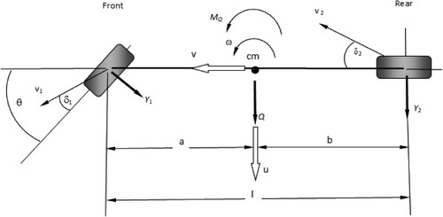
The equations of motion for the two degrees of freedom model are: (1) $\begin{array}{rl}& m(\dot{u}+\mathrm{v\omega })=Y_1+Y_2+Q\end{array}$(1) (2) $\begin{array}{rl}& J\dot{\omega }=a{Y}_1-b{Y}_2+M_Q\end{array}$(2) where:

Y₁, Y₂ are the side forces acting on the front and rear tyres

${\delta }_1$, ${\delta }_2$ are the reduced slip angles at the front and rear tyres, respectivelyQ is the external lateral aerodynamic force applied to the car at the centre of mass

M_Q is the external yaw moment due to Q acting about the vertical axis through the centre of mass

u is the lateral velocity at the centre of mass of the vehicle

v is the longitudinal velocity at the centre of mass of the vehicle

v₁, v₂ are the velocities at the centre of the front and rear axles respectively

ω is the angular velocity (yaw rate) of the vehicle

J is the mass moment of inertia of the vehicle in the yaw plane

a is the distance of the centre of mass from the front axle

b is the distance of the centre of mass from the rear axle

m is the gross mass of the vehicle

l is the wheelbase (a+b)

θ is the steering angle at the front tyres

The non-linear model of the vehicle includes the non-linear descriptions of the lateral tyre forces that are dependent on the slip angles δ₁ and δ₂ at the front and rear tyres. These are given by: (3) $\begin{array}{rl}{\delta }_1& =\theta -\frac{u+\mathrm{a\omega }}{v}\end{array}$(3) (4) $\begin{array}{rl}{\delta }_2& =\frac{-u+\mathrm{b\omega }}{v}\end{array}$(4)

Linearised expressions have been used in Equations (3) and (4) because the variation from the exact value of slip angle is no more than three percent if the slip angle is less than 17 degrees.

The vertical loads, N₁ at the front axle and N₂ at the rear axle are given by: (5) $\begin{array}{rl}{N}_1& =\frac{\mathrm{mgb}}{l}\end{array}$(5) (6) $\begin{array}{rl}{N}_2& =\frac{\mathrm{mga}}{l}\end{array}$(6)

Introducing the parameters${\overline{Y}}_i$, where i is either 1 for the front axle or 2 for the rear axle, and  $q$, $\mu$ converts the equations to a non-dimensional form in order to generalise the solutions. (7) $\begin{array}{rl}{\overline{Y}}_i& =\frac{Y_i}{N_i}\end{array}$(7) (8) $\begin{array}{rl}{\overline{k}}_i& =\frac{k_i}{N_i}\end{array}$(8) (9) $\begin{array}{rl}q& =\frac{Q}{\mathrm{mg}}\end{array}$(9) (10) $\begin{array}{rl}\mu & =\frac{M_Q}{\mathrm{mgab}}l\end{array}$(10) where:

${\overline{Y}}_i$ are the non-dimensional side forces acting at the front and rear wheels

${\overline{k}}_i$ are the non-dimensional tyre cornering stiffnesses of the front and rear wheels

g is the acceleration due to gravity.

The following inputs are introduced here, including

$\theta ={\theta }_{(q)}$, which is the steering input required to stabilise straight-line motion in the presence of the external non-dimensional lateral force q,

$\theta ={\theta }_{(q,\mu )}$, which is the steering input to stabilise straight-line motion in the presence of the external non-dimensional lateral force q and the non-dimensional moment µ. Both inputs are obtained in an analytical form later in the paper.

It should be emphasised that more detailed methods of representing a vehicle model and simulation can make use of a multibody systems approach [31]. Although relatively simple, the bicycle model used in this paper still allows for investigations of extreme and dangerous driving situations towards the limit handling performance of the vehicle. This approach facilitates the prediction of the vehicle driving commands required to maintain control of the vehicle and then can be extended to multibody dynamics in following studies. Such technical problems includes one of influencing the dynamics of the vehicle while it is subjected to the external lateral side force and the resulting moment about the vertical axis of the vehicle, which is the subject-matter in the paper. In the formulation of the problem, the magnitude of the external force and the associated moment are treated as parameters that can vary as a function of the turn angle at the front wheels and the longitudinal speed of the vehicle.

Within the extended space of model parameters in the proposed approach, it is possible also to analyse the set of states for a nonlinear driver model, the boundaries of stability in the parameter space, and the selection of the required steering inputs to maintain stable control of the vehicle.

An important element of the analysis is the assessment of the maximum possible values of the external disturbance for which the driver’s control input is still possible. However, the real ‘safe’ values of the force perturbations are much more complex and are associated with stability diagrams as will be discussed further in this paper.

When visualising the results of the proposed bifurcation approach, idealised nonlinear monotonous dependencies of the tyre lateral forces are used in the non-linear form of arctangent. This does not exclude the possibility of constructing an appropriate bifurcation set for the case of lateral tyre forces specified, for example, by the Magic Formula; in such a case, a numerical procedure to obtain an inverse function and its approximation by a spline can be in use. However, for monotone dependencies of lateral forces the divergent vector field of the vehicle system model is negative in all of the phase-plane, and the Bendixson-Dulac theorem (known also as Bendixson’s criterion) [32] guarantees that there are no limit cycles (Hopf’s bifurcation) in that system.

3. Construction and analysis of the bifurcation diagram

In this section, a special case for the vehicle model described by Equation (1) is considered which accounts only for the lateral external force Q. The resulting moment M_Q is taken to be zero at this stage. The equations that determine the steady-state behaviour in the presence of the lateral external force Q only are: (11) $\begin{array}{rl}\frac{\mathrm{V\omega }}{g}& =\overline{Y_1}\frac{b}{l}+\overline{Y_2}\frac{a}{l}+q\end{array}$(11) (12) $\begin{array}{rl}\overline{Y_1}-\overline{Y_2}& =0.\end{array}$(12)

From Equation (12) it is possible to introduce a new function [9,10] as shown in Equation (13): (13) $\begin{array}{r}\overline{Y}=\overline{Y}({\delta }_2-{\delta }_1):\overline{Y}={\overline{Y}}_1({\delta }_1)={\overline{Y}}_2({\delta }_2).\end{array}$(13) This is the starting point in the implementation of the geometrical approach developed by Pevsner and Pacejka for the analysis of a set of stationary states nonlinear model vehicle. The function $\overline{Y}=\overline{Y}({\delta }_2-{\delta }_1)$ is defined by the dimensionless dependence of forces on the slip angle at the front and rear axles, as shown in Figure 2.

Figure 2. Graphical representation obtained using the Pevsner function $\overline{Y}=\overline{Y}({\delta }_2-{\delta }_1)$ for the geometrical analysis of a set of stationary states for the vehicle model described by Equations (1) and (2).

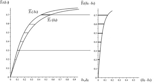
The input (δ₂-δ₁) in Equation (13) is the difference between the slip angles at the tyres for the rear and front axles. After introducing the function $\overline{Y}=\overline{Y}({\delta }_2-{\delta }_1)$, then Equation (11) can be represented as: (14) $\begin{array}{r}\frac{\mathrm{V\omega }}{g}=\overline{Y}({\delta }_2-{\delta }_1)+q\end{array}$(14) where: (15) $\begin{array}{r}\omega =\frac{V(\theta +{\delta }_2-{\delta }_1)}{l}\end{array}$(15) and: (16) $\begin{array}{r}\overline{Y}({\delta }_2-{\delta }_1)=\frac{V^2}{\mathrm{gl}}(\theta +{\delta }_2-{\delta }_1)-q\end{array}$(16)

As an example to illustrate the use of Equation (16) for the geometric analysis of the set of stationary states of the vehicle model it will further be shown in section 7 by using the Pevsner-Pacejka method and the defining function $\overline{Y}=\overline{Y}({\delta }_2-{\delta }_1)$ geometrically built in Figure 2. Note that various options for introducing the function can be proposed, however, the problem is to determine an analytical closed-form expression for Equation (13). The absence of such an analytical representation for Equation (13) was the main obstacle for further analysis of the non-linear vehicle model on the basis of bifurcation theory and the applied catastrophe theory. Therefore, the second important step for the implementation of the bifurcation approach is the transition to an analytical form of the defining equation. This becomes possible by introducing analytical inverse functions for the initial dependencies of the lateral forces Y _i (δ_i). This is further achieved using a monotonous arctangent function as follows: (17) $\begin{array}{r}{\overline{Y}}_i=2{\kappa }_i\arctan (0.5{\overline{k}}_i{\delta }_i\pi /{\kappa }_i)/\pi \end{array}$(17) which leads to: (18) $\begin{array}{r}{G}_i=2\tan (0.5\pi \overline{Y}/{\kappa }_i){\kappa }_i/\pi {\overline{k}}_i\end{array}$(18)

where:

${\overline{k}}_i$ is the non-dimensional tyre cornering stiffness of the front and rear wheels

${\kappa }_i$ is the peak friction coefficient in lateral direction of the front and rear tyres

G_i is the inverse function for lateral axle forces acting at the front and rear tyres

The first step towards the analytical representation of the dependency $\overline{Y}({\delta }_2-{\delta }_1)$ will be the transition to the functions: (19) $\begin{array}{r}{\delta }_2=G_2(\overline{Y})\end{array}$(19) and: (20) $\begin{array}{r}{\delta }_1=G_1(\overline{Y})\end{array}$(20) These are the inverse functions of the original functions ${\overline{Y}}_1={\overline{Y}}_1({\delta }_1)$ and ${\overline{Y}}_2={\overline{Y}}_2({\delta }_2)$ . The use of Equations (18) through (20) leads to the following analytical representation of the slip angle difference: (21) $\begin{array}{r}{\delta }_2-{\delta }_1=G(\overline{Y})\end{array}$(21) which is the inverse of the function $\overline{Y}=\overline{Y}({\delta }_2-{\delta }_1)$, as the difference between the two functions ${\delta }_2=G_2(\overline{Y})$ and ${\delta }_1=G_1(\overline{Y})$.

In a case when an analytical representation of the dependence $\overline{Y}=\overline{Y}({\delta }_2-{\delta }_1)$ cannot be determined, the following expression can be used: (22) $\begin{array}{r}G(\overline{Y})=\frac{\mathrm{gl}}{V^2}(\overline{Y}+q)-\theta \end{array}$(22) The stationary states for the system defined in Equations (1) and (2) correspond to the intersecting points of the ‘movable’ line $\frac{\mathrm{gl}}{V^2}(\overline{Y}+q)-\theta$ and the ‘unmovable’ curve $G(\overline{Y})$ defined in Equation (22). This approach is similar to the Pevsner-Pacejka method based on Equation (16) considering the intersection of the ‘movable’ line $\frac{V^2}{\mathrm{gl}}(\theta +{\delta }_2-{\delta }_1)-q$ and the ‘unmovable’ curve$\overline{Y}({\delta }_2-{\delta }_1)$.

From the geometric interpretation of the solution of Equation (22) we can find that its discriminant manifold is a curve that is dual to the curve $G(\overline{Y})$ as previously shown in [33]. It is the locus on the plane of the control parameters (V, θ) where the line represented by $\frac{\mathrm{gl}}{V^2}(\overline{Y}+q)-\theta$ is tangent to the curve represented by $G(\overline{Y})$. Figure 3 known as a controllability diagram illustrates the geometric interpretation of the divergent loss of stability of the stationary regime. A multiple regime occurs when the line represented by $\frac{\mathrm{gl}}{V^2}(\overline{Y}+q)-\theta$ and the curve represented by $G(\overline{Y})$ are tangent. With a parallel displacement of the straight line due to a change in the angle θ, the multiple regimes at the point of intersection (Figure 3) either disappear or separates into two simple (single) regimes. One of them is a stable node, and the second unstable one is a saddle. This conclusion follows from the general provisions of the qualitative theory of dynamical systems [23,32] as described, for example, in [30].

Figure 3. The points of intersection between a moving straight line and a fixed curve indicate a divergent loss of stability in the corresponding multiple stationary regime, i.e. a bifurcation of a fold.

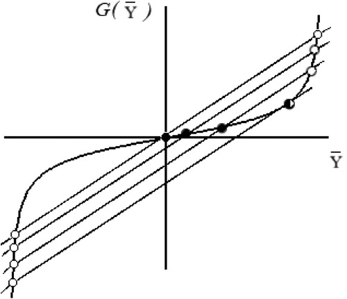
To determine the stability of a stationary regime for some fixed values of control parameters using the controllability diagram (Figure 3), it is necessary to know the ‘prehistory’ of at least one stationary mode. For example, Figure 3 illustrates the evolution of three stationary modes corresponding to certain parameters shown by the black bullets. These regimes are characterised by the subcritical speed of rectilinear motion V (when V is less than the critical value) with zero steering angle at the wheels and by the magnitude of the lateral force which is also to be considered equal to zero at zero steering angle. The change in the position of the moving straight line $\frac{\mathrm{gl}}{V^2}(\overline{Y}+q)-\theta$ (see Figure 3) in the presence of a constant lateral force can be taken into account by holding the turn angle of the front wheels constant and equal to $\mathrm{\Delta }\theta =-\frac{\mathrm{gl}}{V^2}q$. In such a case, the equation of the moving straight line will take the form $\frac{\mathrm{gl}}{V^2}\overline{Y}-(\theta +\mathrm{\Delta \theta })$. Then the central stationary mode (at the origin in Figure 3) corresponds to the stable rectilinear mode, if the slope of the moving straight line is greater than the slope of the fixed curve at the origin $\frac{\mathrm{gl}}{V^2}>\frac{1}{{\overline{k}}_2}-\frac{1}{{\overline{k}}_1}\Rightarrow V^2<\frac{{\overline{k}}_1{\overline{k}}_2\mathrm{gl}}{{\overline{k}}_1-{\overline{k}}_2}$. When the parameter $\theta$ changes, the stable rectilinear regime transforms into a stable circular mode (adjacent modes on the controllability diagram are shown as solid circles) until the multiple modes are realised. The stationary regime, with which the stable circular regime merges, is a saddle singular point. Taking into account the details of its ‘prehistory’, it can be concluded that for all previous positions (in right part of first quadrant) the asymmetric stationary regimes of the vehicle were unstable (saddle singular points).

If we consider a change in the steering angle in the opposite direction (i.e. in the negative direction), then it can be concluded that the stationary modes to the left of the central rectilinear mode are also saddle modes. However, in the presence of a constant lateral force, the symmetry of the critical values of the left and right angles are lost. It should be noted, that a geometrical analysis of the set of stationary states of the system based on the Pevsner-Pacejka approach of the determining Equation (16) would be obtained if Figure 3 was reflected relative to the bisector of the first and third quadrants. This would occur as the transition from Equation (22) to Equation (16) is a transition to the inverse functions in the left and right sides of the Equation (22).

The inflection points of the original curve $G(\overline{Y})$ will correspond to the cusps on the dual [33] curve. In the parametric form, the dual curve is given by the system described in Equations (23)–(24). (23) $\begin{array}{rl}\frac{\mathrm{gl}}{V^2}& =G^{\mathrm{\prime }}(\overline{Y})\end{array}$(23) (24) $\begin{array}{rl}\theta & =G^{\mathrm{\prime }}(\overline{Y})(\overline{Y}+q)-G(\overline{Y})\end{array}$(24) All the dual points on this curve determine the critical value of the control parameters (θ, V), referred to below as the bifurcation set of the control parameters. The loss of divergent stability of the stationary states can only occur if the control parameters lie on the bifurcation curve (the critical set of the parameters). In this case, where the moving straight line touches the curve, as shown in Figure 3, we have a multi-fold steady state. The most typical situation is when two-fold stationary states are observed (the case of a simple intersection of the straight line with the non-linear curve). As shown in Figure 4, almost all points of the bifurcation correspond to this situation of the two-fold stationary states, except for the cusp, where three-fold stationary states are realised.

Figure 4. Bifurcation diagram (solid curve) defined by the Equations (23)-(24) and the (dash curve) obtained using the numerical continuation method.

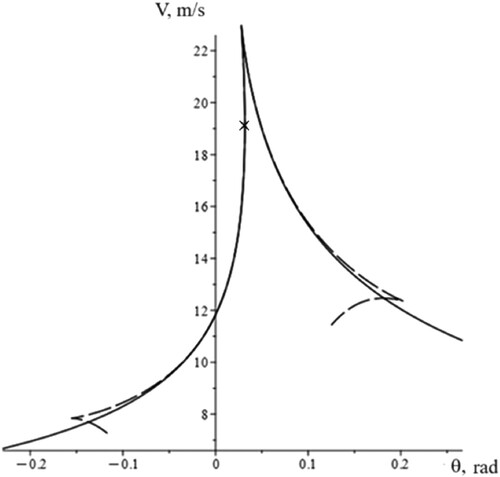
If the representative point (θ, v) in the parameter plane intersects the critical (bifurcation) set, then the number of stationary states changes by two units (a pair of states appears or disappears). For example, in Figure 3, the change could be from 3 to 1 (meaning that two stationary states disappear) or from 1 to 3 (two stationary states appear). If we are dealing with the disappearance of a twofold stationary state (fold bifurcation [23]), then one of them loses stability along with itself. If we are dealing with the appearance of a double stationary state, then one stable stationary state arises in the system. For example, if we have a stable stationary state and a change of the control parameters it become three-fold and after bifurcation (cusp bifurcation) remains one simple stationary regime. This indicates that the additional two stationary states are unstable, and that our stable regime and one unstable regime disappear in the resulting bifurcation. As such, this is the mechanism for the loss of the stability of the stationary state when it exists after divergent bifurcation.

For the modelling and analysis purposes described earlier in this paper, a sample set of a mid-size sedan was used. This included the following parameters: m = 1317 kg, J = 3050 kg^.m², κ₁= 0.8, κ₂= 0.8, a = 2.3 m, b = 2.7 m, g = 9.81 m/s², Q = 0.3*m*g N, k₁= 23000 N, k₂= 15000 N. Note that the lateral force Q is taken to be 30% of the vehicle weight. Figure 4 shows the corresponding bifurcation diagram for this car model.

In Figure 4 bifurcation diagram (the dashed curve) are used to obtain a base continuation method with the factor cos (θ) and the dimensionless force Ȳ₁, which we neglected in the original system (11)-(12), shown here by the dash curve line.

The x-sign on the bifurcation diagram shown in Figure 4, defined by the intersection of the moving straight line $\frac{\mathrm{gl}}{V^2}(\overline{Y}+q)-\theta$ and the curve $G(\overline{Y})$, points to a loss divergent stability of rectilinear motion when θ_q = 0.0316 rad and v = $V^{\times }=$ 19.11 m/s. The numerical continuation method described in [19,21] can indicate the difference in the results obtained using analytical approach with a simple bicycle model from those found using a model that takes into account the factor cos(θ) of the force Ȳ_1. The correspondent point on the dashed has coordinates that correspond with $\theta$ = 0.0315 rad and v = $V^{\times }=$19.14 m/s and was taken as a starting point for the numerical construction of a bifurcation curve using the continuation method for the system described by Equations (11)-(12) modified to account for the factor cos (θ) of the force Ȳ₁.

It should be noted that in the case where symmetry in the model of the vehicle is not present, for example under the action of an external lateral force and the resulting moment of that force, then the search for a starting point becomes an additional and difficult task using the method of continuation. This makes the analytical method more practical for a qualitative analysis and the understanding of the mechanical processes in such cases.

4. Stabilisation of the straight-line motion of the vehicle model in the presence of the external lateral force Q acting through the vehicle centre of mass (M_Q = 0)

In this section, we consider the steering correction that is required to return a vehicle to stable straight-line motion when it is subjected to a constant external lateral force. In this case, the resulting centripetal acceleration is equal to the sum $(\overline{Y}+\overline{Q})$ and, therefore, to achieve straight-line motion the condition $\overline{Y}+\overline{Q}=0$ must be met.

Hence we have, (25) $\begin{array}{r}\overline{Y}=-q\to {\delta }_2-{\delta }_1=G(-q)\end{array}$(25) If yaw motion is also to be eliminated, $\omega =0$, then it must also be true that the condition $\theta =-({\delta }_2-{\delta }_1)$ exists.

This gives: (26) $\begin{array}{r}{\theta }_{(q)}=-G(-q)\end{array}$(26) Under the linear lateral tyre forces, the proposed control function coincides with the known ratio (27) derived in some references, for example [18,34]. For the case of an odd function $G(\overline{Y})$ we have ${\theta }_{(q)}=G(q)$. The linearisation of this function near zero gives: (27) $\begin{array}{r}{\theta }_{(q)}=\frac{{\overline{k}}_1-{\overline{k}}_2}{{\overline{k}}_1{\overline{k}}_2}q\end{array}$(27)

Equation (26) can be refined by introducing the factor cos (θ) with a dimensionless force Ȳ₁, which we neglected in the original system described by Equations (1) and (2). If we introduce the factor cos (θ) we obtain: (28) $\begin{array}{rl}{\overline{Y}}_1({\delta }_1)& =-q/\text{cos}({\theta }^{(0)})\end{array}$(28) (29) $\begin{array}{rl}{\overline{Y}}_2({\delta }_2)& =-q\end{array}$(29)

We can use an iterative process to determine a more accurate value of the angle $\theta$. As a start we can take ${\theta }^{(0)}=0$.

From Equations (28) and (29) and the arguments ${\delta }_i^{(0)}$, we obtain the first approximation: (30) $\begin{array}{rl}{\delta }_2^{(0)}& =G_2(-q)\end{array}$(30) (31) $\begin{array}{rl}{\delta }_1^{(0)}& =G_1(-q/\text{cos}({\theta }^{(0)}))=>{\theta }^{(1)}={\delta }_1^{(0)}-{\delta }_2^{(0)}\end{array}$(31)

This result is consistent with Equation (11) and can be further refined on the basis of iterations to give ${\theta }_{(q)}=0.0315$ rad. The requirement for the presence of an analytical inverse function is not essential in this case. As a result, we get a condition $({\omega }^{\ast }=0,$ $u^{\ast }\ne 0)$, and since the vehicle will have a body slip angle: (32) $\begin{array}{r}{\psi }^{\ast }:\tan ({\psi }^{\ast })=u^{\ast }/v\end{array}$(32)

In order to establish straight-line rectilinear motion, it is necessary to correct the heading angle by the value $\mathrm{\Delta \Psi }=-{\psi }^{\ast }$. The stabilisation of this motion is controlled by the steering angle $\theta$ as solved below: (33) $\begin{array}{r}\frac{\omega }{{(u^2+v^2)}^{\frac{1}{2}}}+\frac{\dot{u}\cdot v}{{(u^2+v^2)}^{\frac{3}{2}}}=K_r\end{array}$(33) where $\dot{u}$determines the lateral acceleration component of the vehicle centre of mass from the first equation of system (1) and $K_r$ is the path curvature (in this case of straight-line motion $K_r$ = 0). Figure 5 shows the generated control angle θ based on a solution of Equation (33), needed for the stabilisation of straight-line motion using a non-linear model of the vehicle.

Figure 6 provides a planar view for the forward trajectory of the vehicle and the progressive stabilisation of straight-line motion generated by the steering angle $\theta (t)$, represented in Figure 5.

Figure 5. Steering Angle θ as function of time for the realisation of straight-line motion where $\theta (t)$ → ${\theta }_{(q)}=0.0315$rad.

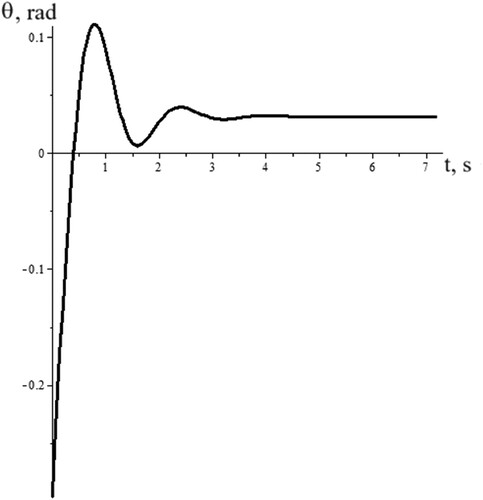
Figure 6. The stabilisation of straight-line motion generated by the steering angle $\theta (t)$ as solved by Equation (33).

The vehicle motion after correcting the heading angle by the value $\mathrm{\Delta \Psi }=\text{arctan}(-u^{\ast }/v)$ to compensate the body slip angle is shown in Figure 6.

5. Construction of the bifurcation diagram of the vehicle model in the presence of the external lateral force Q and the associated moment M_Q acting about a vertical axis at the vehicle mass centre

The condition where no moment is present (M_Q ≠ 0) is described above in Equations (23)–(24). We can consider now the case where an additional external moment M_Q forces acting about a vertical axis through the centre of mass exists.

For this case, the defining equation is: (34) $\begin{array}{r}\overline{Y}({\delta }_2-{\delta }_1,\mu )=\frac{v^2}{\mathrm{gl}}(\theta +{\delta }_2-{\delta }_1)-q-a\frac{\mu }{l}\end{array}$(34) where:

$\overline{Y}({\delta }_2-{\delta }_1,\mu )$: ${\overline{Y}}_1={\overline{Y}}_2-\mu ;$ $q=Q/(m\text{g})$ – dimensionless value of the external lateral forces

$\mu =M_Q\cdot l/(m\text{g}\mathrm{ab})$ – dimensionless value of the moment resulting from the external lateral forces

The form of ‘stationary’ curve $\overline{Y}({\delta }_2-{\delta }_1,\mu )$ is related to the magnitude of the external moment. The generalisation of Equation (22) is obtained formally, leading to the inverse functions in the left and right parts as shown in Equation (35) (35) $\begin{array}{r}G(\overline{Y,}\mu )=\frac{\mathrm{gl}}{v^2}\left(\overline{Y}+q+a\frac{\mu }{l}\right)-\theta \end{array}$(35) The conditions for touching the ‘moveable’ line $\frac{\mathrm{gl}}{v^2}\left(\overline{Y}+q+a\cdot \frac{\mu }{l}\right)$ with the ‘stationary’ curve $G(\overline{Y,}\mu )$ correspond to the implementation of multiple stationary states (divergent bifurcations), represented by the system described in Equations (36) to (37) (36) $\begin{array}{rl}{v}^2& =\frac{\mathrm{gl}}{G^{\mathrm{\prime }}(\overline{Y,}\mu )}\end{array}$(36) (37) $\begin{array}{rl}\theta & =G^{\mathrm{\prime }}(\overline{Y},\mu )\left(\overline{Y}+q+a\frac{\mu }{l}\right)-G(\overline{Y},\mu ),\end{array}$(37) where the derivative is taken with respect to the argument $\overline{Y}$.

This provides the bifurcation set of the non-linear model of the vehicle (stability diagram) in parametric form (here the Ȳ independent parameter).

The Equations (35), (36), (37) where $G(\overline{Y},\mu )=G_2(\overline{Y}+\mu )-G_1(\overline{Y})$ can be written in a more symmetrical form, in this case with the function $\overline{Y}({\delta }_2-{\delta }_1,\mu )$: ${\overline{Y}}_1+a\cdot \frac{\mu }{l}={\overline{Y}}_2-b\cdot \frac{\mu }{l}$.

Then Equation (34) becomes: (38) $\begin{array}{r}\overline{Y}({\delta }_2-{\delta }_1,\mu )=\frac{v^2}{\mathrm{gl}}(\theta +{\delta }_2-{\delta }_1)-q\end{array}$(38) where $\overline{Y}({\delta }_2-{\delta }_1,\mu )+q=\overline{a_y}=\frac{\omega \cdot v}{g}.$

Equation (35) can be transformed to Equation (39) with a new independent parameter $\overline{a_y}$_, this being the dimensionless centripetal lateral acceleration acting at the centre of mass of the vehicle. (39) $\begin{array}{r}G(\overline{a_y},q,\mu )=\frac{\mathrm{gl}}{v^2}\cdot \overline{a_y}-\theta \end{array}$(39) where $G(\overline{a_y},q,\mu )=G_2\left(\overline{a_y}-q+b\frac{\mu }{l}\right)-G_1\left(\overline{a_y}-q-a\cdot \frac{\mu }{l}\right).$

If $\overline{a_y}=v^2/(R\text{g})$ then from Equation (39) we get the generalisation for the equation of handling described by Equation (40): (40) $\begin{array}{r}\theta =l/R-G(\overline{a_y},q,\mu )\end{array}$(40)

The system of Equations (36) to (37) that define the conditions for a of loss of divergent stability stationary states leads to the system of equations (41) and (42). (41) $\begin{array}{rl}{v}^2& =\lg /G^{\mathrm{\prime }}(\overline{a_y},q,\mu )\end{array}$(41) (42) $\begin{array}{rl}\theta & =G^{\mathrm{\prime }}(\overline{a_y},q,\mu )\cdot \overline{a_y}-G(\overline{a_y},q,\mu ),\end{array}$(42) where the derivative is taken with respect to the argument $\overline{a_y}$.

After comparing Equation (42) with Equation (40) we obtain the condition for a divergent loss of stability on the handling curve. This condition takes place if Equation (43) has a real solution ${\overline{a_y}}^{\ast }$. (43) $\begin{array}{r}l/R=G^{\mathrm{\prime }}(\overline{a_y},q,\mu )\cdot \overline{a_y}\end{array}$(43) The bifurcation set of the control parameters and curve of handling would be more suitably plotted using the system Equations (40), (41) and (42).

Figure 7 shows the development of the base analytical Equations (40–42).

Figure 7. Analysis of divergent loss stability on the handling curve (with turning radius of R = 30 m); The long-dash curves are the handling curves and indicate the change in steering angle required for the vehicle to remain on a circlular trajectory of fixed radius if a change in the speed V occurs. The smooth solid curves are the bifurcation sets with the critical values of the control parameters (θ, V) corresponding to a divergent loss in stability for the stationary states of the system: (a) represents q =  μ = 0; (b) represents q =  0.3, μ = 0; (c) represents q =  0.3, μ = 0.03.

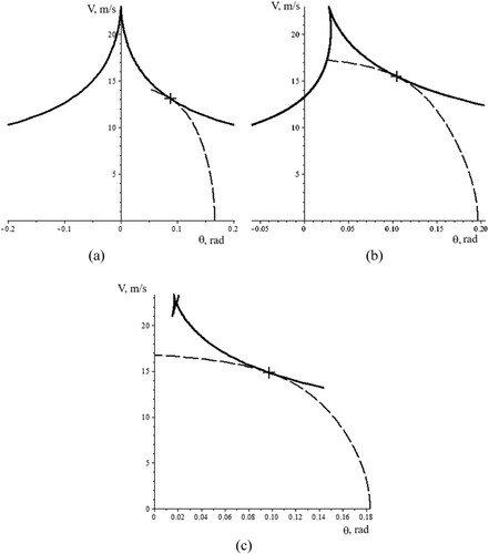
Here we can see a change in the configuration of the bifurcation set and the handling curve, for different values of the lateral force q and the external moment μ, at points where the handling curve is tangent to bifurcation set. This occurs when there is a loss of divergent stability for the stationary circular regime and there is a fixed radius of curvature R = 30 m.

The coordinates for the points where there is a divergent loss of stability on the handling curve for R = 30 m occur when the vehicle control parameters (θ, V) are [0.0881 rad, 13.07 m/s], [0.1047 rad, 15.46 m/s], [0.0974 rad, 14.84 m/s] consequently. Following these critical points on the control parameters plane, the vehicle parameters enter another stable stationary regime with a radius of curvature that is different from the 30 m. This is shown for the cases (a) and (b) in Figure 7 where a safe recovery of stability exists. Case (c) in Figure 7, however, shows a dangerous loss stability where the vehicle is not able to return to any stable stationary regime.

6. The graphical interpretation of stability analysis of the stationary states and qualitative conclusions about the counteraction of the resultant of the external lateral forces Q (M_Q = 0)

We can illustrate the characteristics of the implementation of the straight-line motion of the vehicle when subjected to a lateral force $Q$ based on the Pevsner-Pacejka’s graph – analytical method in the plane of variables $({\delta }_2-{\delta }_1,$ $\overline{Y}({\delta }_2-{\delta }_1))$. We will analyse the case of the subcritical value of the longitudinal speed $v<V^{\times }$.

The diagrams shown in Figure 8 (a), (b) and (c), present the characteristic cases of the implementation of a set of stationary states for the system that corresponds to the intersecting points of the moving straight-line with the stationary curve $\frac{V^2}{\mathrm{gl}}(\theta +{\delta }_2-{\delta }_1)-q$ and the stationary curve $\overline{Y}({\delta }_2-{\delta }_1)$. This occurs in accordance with the geometric interpretation of the defining Equation (16). The straight-line stationary regime (ω = 0) corresponding to $O_1$ is achieved by the appropriate choice of the parrying angle ${\theta }_{(q)}$. In Figure 8, straight line 1 needs to be displaced by the angle ${\theta }_{(q)}$ to a new position, shown by line 2, in order to counter the lateral force. These two straight lines are parallel to each other.

Figure 8. Graphical illustration of corrective steering angles under external lateral force; (a): the condition ${\overline{k}}_1>{\overline{k}}_2$, ${\kappa }_1={\kappa }_2$; (b): the condition ${\overline{k}}_1<{\overline{k}}_2$, ${\kappa }_1={\kappa }_2$; (c) and (d): ${\overline{k}}_1>{\overline{k}}_2$, ${\kappa }_1<{\kappa }_2$.

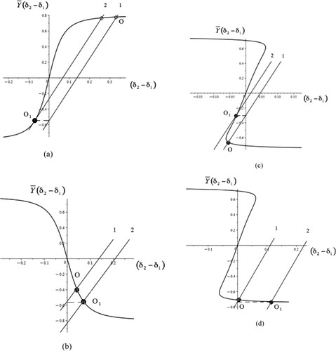
The intersection of line 1 with the curve $\overline{Y}({\delta }_2-{\delta }_1)$ is identified as the point O in Figure 8. This point corresponds to the stationary regime where there is lateral force $Q$ with $\theta =0$. It can be seen that line 1 crosses the y-axis at the point (0, $-q$). Since the yaw rate during straight-line motion is equal to zero ω = 0, as developed in Equation (15), then from equations (15) and (16) we have a condition that must be satisfied for straight-line motion to exist: (44) $\begin{array}{r}\overline{Y}({\delta }_2-{\delta }_1)=-q\end{array}$(44) Therefore, we move parallel to line 1 to the state where the intersection with the curve $\overline{Y}({\delta }_2-{\delta }_1)$ occurs at the position $q$. This is position 2, which is the abscissa of $O_1$ up to a point that coincides with the value of the required corrective angle ${\theta }_{(q)}$ that is consistent with Equation (42).

Now we demonstrate some results of a qualitative nature about the corrective side force required to achieve straight-line motion. The front wheels steer through an angle of ${\theta }_{(q)}$(line 2). The situation when ${\theta }_{(q)}>0$ represents the wheels turning towards the action of the force $Q$ for the condition ${\overline{k}}_1>{\overline{k}}_2$ (this relationship between the cornering stiffness at the front and rear tyres ensures that the vehicle will oversteer) as shown in Figure 8 (a). The situation where the wheels steer away from the action of the force Q and the condition ${\overline{k}}_1<{\overline{k}}_2$ exists is shown in Figure 8 (b). The functional dependence of the corrective angle as a function of the dimensionless lateral force coincides with the solution of the $\overline{Y}({\delta }_2-{\delta }_1)$ equation. The counteraction of the lateral force is only possible for the case $|q|<\text{min}({\kappa }_1,{\kappa }_2).$

In the case illustrated by Figure 8 (a) point $O_1$ corresponds to the stable straight-line regime until v < $V^{\times }$ (v is less critical speed $V^{\times }$). The stable straight-line regime shown in Figure 8 (b) occurs for any value of the parameter v.

The curves shown in Figure 8 c.

However, there are some cases where the curve has the form shown Figure 8 (c) and (d), cases${\overline{k}}_1>{\overline{k}}_2,$ ${\kappa }_1<{\kappa }_2$. For the case presented in Figure 8 (c) and (d) the same situation exists as in the case shown in Figure 8 (b), where the straight-line regime at the point $O_1$ remains stable during the whole interval of change in the scalar lateral force over the range $|q|<\text{min}({\kappa }_1,{\kappa }_2).$

We can now consider the qualitative difference in correcting the lateral force by introducing the steering angle of the front wheels for cases $({\overline{k}}_1-{\overline{k}}_2)\cdot ($ ${\kappa }_1-{\kappa }_2)<0$. In the former case (Figure 8, (c)) the angle ${\theta }_{(q)}$ > 0 is for the situation $({\overline{k}}_1-{\overline{k}}_2)>0$ and ${\theta }_{(q)}<0$ is for the situation $({\overline{k}}_1-{\overline{k}}_2)<0$. When $Q>0$ and the vehicle is exposed to the lateral force $Q^{\ast }$ applied at the centre of mass it is not possible to achieve straight-line motion due to a corrective steering input using a linear model of the vehicle. In the second case (Figure 8, (d)), the sign of ${\theta }_{(q)}$depends on the value of $Q$ and an increase in the scalar force $Q$.

It can be seen in Figure 8 (d) that there is a value of the lateral force $q^{\ast }$ that is numerically equal to the length of the segment cut off by the fixed curve on the ordinate axis, such that the required corrective angle ${{\theta }_{(q)}}^{\ast }=0$. This means the vehicle exposed to the lateral force $q^{\ast }$, applied at the centre of mass, can travel in a straight line without any steering input.

7. The graphical interpretation of the stability analysis of the stationary states and conclusions about the counteraction of the external lateral forces Q and the resulting moment M_Q

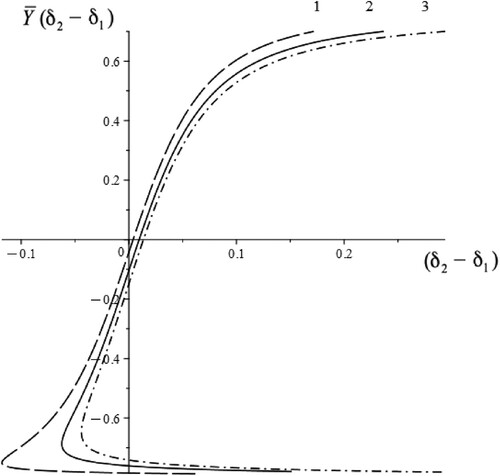
The geometrical pattern for the selection of the corrective steering input required to achieve straight-line travel for the case with an additional external moment about the vertical central axis does not change. We can see in Figure 9 a more complicated shape of the curve for $\overline{Y}({\delta }_2-{\delta }_1,\mu )$ with different values of the moment parameter μ.

Figure 9. Graph of $\overline{Y}({\delta }_2-{\delta }_1,\mu )$ for different values of parameter μ $(1.{\mu }_1=0.01;2.{\mu }_2=0.0242;3.{\mu }_3=0.0342)$.

For the case shown in Figure 10 where $\mu =0.0242$, line 2 corresponds to a stable circular regime (point$O_1$), and another point indicated (white disks) where the circular regime is unstable. This is consistent with the general qualitative methods of analysis of dynamical systems on a phase plane [32]. The geometrical analysis of stability of a stationary state can be used next in a simple form. The state of stability does not change until there is a change in the control parameters θ or v. It does not become complex and connect with another stationary states.

Figure 10. Determination of the corrective steering angle for straight-line motion with a moment of the external force acting about the centre of mass vehicle (μ = 0.0242, q = 0.3, v = 18 m/s).

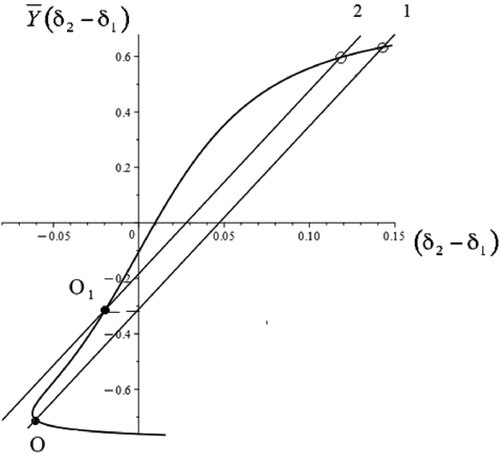
Figure 10 shows that with an increase in the parameter $\theta$ the stable regime indicated by point O₁ meets the unstable regime at point of intersection between line 2 and the stationary curve $\overline{Y}({\delta }_2-{\delta }_1,\mu ).$ One from these is a stable state and another is an unstable state (saddle). A stationary state that lies on the linear part of the curve $\overline{Y}({\delta }_2-{\delta }_1,\mu )$ is stable if the slope of the moving straight-line $\frac{v^2}{\mathrm{gl}}(\theta +{\delta }_2-{\delta }_1)-q-a\cdot \frac{\mu }{l}$ is less than the slope of the curve $\overline{Y}({\delta }_2-{\delta }_1,\mu )$ at the point of intersection. Since line 1 has the same gradient and is parallel to line 2 there is one stable state at point O and one unstable stationary state as indicated (white disks).

A further consider of a condition to realise straight-line motion for a general case when there is an external lateral force and resulting moment acting on the vehicle is possible. From Equation (34), which defines a set of stationary states where ω = 0, and taking into account Equation (15), we get a condition that must comply with the required straight-line regime: (45) $\begin{array}{r}\overline{Y}({\delta }_2-{\delta }_1,\mu )=-q-a\cdot \frac{\mu }{l}\end{array}$(45) This means that line 1, shown in Figure 10, due to the choice of corrective steering angle $\theta$ must be transferred parallel to the position where the intersection point with the curve $\overline{Y}({\delta }_2-{\delta }_1,\mu )$ has the value $-q-a\cdot \frac{\mu }{l}$ at point $O_1$. The abscissa of point $O_1$ up to a position that coincides with the value of the required corrective angle θ. The analytical expression from which you can get the numerical value of the corrective steering angle follows from Equation (35) and is solved with the solution of ${\delta }_2-{\delta }_1$ for the straight-line regime $\theta =-({\delta }_2-{\delta }_1)$. (46) $\begin{array}{r}\theta =-({\delta }_2-{\delta }_1)=-G(\overline{Y},\mu ){|}_{\overline{Y}=-q-a\cdot \frac{\mu }{l}}\end{array}$(46)

This can be refined in the same way as in the case of Equation (26).

If we take ${\theta }^{(0)}=0,$ then solving the system described by Equations (47) and (48) shows that straight-line travel is possible if $\text{min}({\kappa }_1,{\kappa }_2)\ge \text{max}\left(q+a\cdot \frac{\mu }{l},q+b\cdot \frac{\mu }{l}\right)$. (47) $\begin{array}{rl}{\overline{Y}}_1({{\delta }_1}^{(0)})& =\left(-q-a\cdot \frac{\mu }{l}\right)/\text{cos}({\theta }^{(0)})\end{array}$(47) (48) $\begin{array}{rl}{\overline{Y}}_2({{\delta }_2}^{(0)})& =-q+b\cdot \frac{\mu }{l}\end{array}$(48)

Finding the solutions ${{\delta }_i}^{(0)}$ from Equations (47) and (48) we obtain the first approximation: ${\theta }^{(1)}={{\delta }_1}^{(0)}-{{\delta }_2}^{(0)}\text{and so on}\text{(}{{\theta }^{(1)}}_{(q,\mu )}=0.01928,\dots ,{\theta }_{(q,\mu )}=0.01924).$However, the stability of this rectilinear regime is only possible if the velocity does not exceed the limiting value V^× previously determined from Equations (36) and (41). Figure 11 shows the bifurcation set developed using the base analytical Equations (41) and (42); and the analysis is based on the numerical continuation for two parameters (θ, v). This takes into account the factor cos (θ), which was neglected in the original system described by Equations (1) and (2).

Figure 11. (a): Stability diagram with an additional moment of the external lateral forces acting about a vertical axis at the vehicle of mass centre (μ = 0.0242, q = 0.3); (b): Fragment of stability diagram with an additional moment of the external lateral forces acting about a vertical axis at the vehicle of mass centre (μ = 0.0242, q = 0.3).

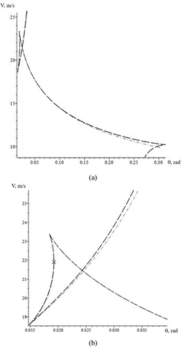
The dashed lines shown in Figure 11 accounts for the cosines of the steering angles and is developed from the base numerical method of continuation for the two parameters $(\theta ,v)$. Figure 11 provides a stability diagram in the parameters plane $(\theta ,v)$, where the x-marker indicates the point with coordinates (${{\theta }^{(1)}}_{(q,\mu )}=$0.01928rad, $V^{\times }=$21.91 m/s) and represents the point where the loss of stability for straight-line motion occurs. This makes it possible to determine the coordinates of the corresponding critical point (see x-marker in Figure 11) based on the analytical relationship given in Equation (41) as follows: (49) $\begin{array}{r}{V}^{\times }=\sqrt{l\text{g}/{G^{\mathrm{\prime }}(\overline{Y},\mu )|}_{\overline{Y}=-q-a\cdot \frac{\mu }{l}}}\end{array}$(49) where $G(\overline{Y},\mu )=G_2(\overline{Y}+\mu )-G_1(\overline{Y}),$ the derivative is taken with respect to the argument $\overline{Y}$.

Or using Equation (39) we get: (50) $\begin{array}{r}{V}^{\times }=\sqrt{l\text{g}/{G^{\mathrm{\prime }}(\overline{a_y},q,\mu )|}_{\overline{a_y}=0}}\end{array}$(50) where $G(\overline{Y},q,\mu )=G_2\left(\overline{a_y}-q+b\cdot \frac{\mu }{l}\right)-G_1\left(\overline{a_y}-q-a\cdot \frac{\mu }{l}\right),$ the derivative is taken with respect to the argument $\overline{a_y}$.

Figure 12 shows a set stationary state for straight-line motion of the vehicle when the loss of divergent stability occurs at a critical value for control parameters that correspond to the position indicated by the x-marker in Figure 11.

Figure 12. The loss of divergent stability for straight-line vehicle motion (μ = 0.0242, q = 0.3) for critical values of the parameters ${{\theta }^{(1)}}_{(q,\mu )}=$0.01928rad, $V^{\times }=$21.91 m/s.

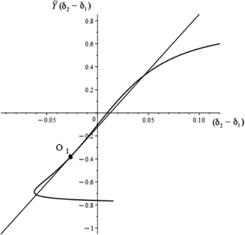
Thus, it has been shown that for a change of control parameters the stability of the stationary states only changes when they merge with another stationary state and form a multiple regime. The straight-line motion stationary state becomes unstable in this situation, and an unstable stationary state becomes stable when v >$V^{\times }$, representing a gradual loss of stability. The bifurcation sets are developed from the analytical Equations (41) and (42) indicating an opportunity for stabilisation with a required steering input.

8. Conclusions

The passive stability of vehicles subjected to a constant lateral force disturbance is an important engineering problem in the daily and normal applications of vehicles.

Note that although the application described here is automotive the work may also contribute to the study of low speed aircraft ground manoeuvring building on other work [35,36]. In this case, the bifurcation approach may be applicable to aircraft during low speed taxiing manoeuvres when it is subject to the laws and theories applicable in ground vehicle dynamics and when there is a need to define the conditions required for straight-line or circular motion on the ground in the presence of lateral wind gusts.

This paper has described the development of an analytical method that can be used to stabilise the straight-line motion of a vehicle and prevent the development of an oversteer response when the vehicle is subject to a lateral external force and a resulting moment acting about a vertical axis through the vehicle centre of mass.

The study made suitable use of the classic linear bicycle model of a two-axle vehicle with steering inputs at the front axle. From the results, a number of conclusions can be made. The first of these is that the shape of the handling curve appears to reflect the geometry. The combination of the two lateral forces, that are functions of the slip angles on the front and rear axles of vehicle, can define the vehicle handling properties for a region with larger slip angles. This can be used in various cases to explain changes in handling properties for large values of lateral acceleration measured at the vehicle’s centre of mass. The second interesting fact is that the value of the corrective steering angle required for the parrying of constant disturbances is dependant only on the lateral forces and do not depend on the speed of vehicle.

Based on the bifurcation approach, which does not require the prior determination of the set of stationary states of the vehicle model, an appropriate method of constructing a critical set of control parameters was implemented (longitudinal speed and steering angle). When intersecting the critical set of parameters, there is a divergent loss of stability of the stationary state, but stability is guaranteed until the moment at which the critical values of the control parameters is reached. The conditions for a divergent of loss stability of the stationary states are found in analytical form and have some potential for the future usage in systems of active control of steering inputs, such as those used in lane keeping, to maintain a stable vehicle trajectory.

This could also have future applications in the algorithms used by autonomous vehicles to determine the steering inputs required to maintain straight-line motion when the vehicle is subject to a side disturbance, such as a strong wind gust.

Future studies will develop this approach for articulated vehicles, additional torque vectoring of the road wheels and road conditions where rapid changes in friction compromise the stable control of the vehicle.

Acknowledgments

The authors express their gratitude to the London Mathematical Society and Isaac Newton Institute Solidarity Programme for the support they have provided for Professor Verbytskyy to conduct the research that has resulted in the authors’ collaborative effort and this research paper.

Disclosure statement

No potential conflict of interest was reported by the author(s).

References

- Farroni F, Russo M, Russo R, et al. A combined use of phase plane and handling diagram method to study the influence of tyre and vehicle characteristics on stability. Veh Syst Dyn. 2013;51(8):1265–1285. doi:10.1080/00423114.2013.797590
- Verbitskii VG, Bezverhyi AI, Tatievskyi DN. Handling and stability analysis of vehicle plane motion. Math Comput Sci. 2018;3(1):13–22. doi:10.11648/j.mcs.20180301.13
- Bobier-Tiu CG, Beal CE, Kegelman JC, et al. Vehicle control synthesis using phase portraits of planar dynamics. Veh Syst Dyn. 2019;57(9):1318–1337. doi:10.1080/00423114.2018.1502456
- Mastinu G, Della Rossa F, Gobbi M, et al. Bifurcation analysis of a car model running on an even surface - A fundamental study for addressing automomous vehicle dynamics. SAE Int J Veh Dyn, Stab, and NVH. 2017;1(2):326–337. doi:10.4271/2017-01-1589
- Liapunov AM. Stability of motion, mathematics in science and engineering, Vol. 30. New York/London: Academic Press; 1966. doi:10.1002/zamm.19680480223
- Ko YE, Lee JM. Estimation of the stability region of a vehicle in plane motion using a topological approach. Int J Veh Des. 2002;30(3):181–192. doi:10.1504/IJVD.2002.002032
- Chen K, Pei X, Ma G, et al. Longitudinal/lateral stability analysis of vehicle motion in the nonlinear region. Mathl Probl Engng. 2016: doi:10.1155/2016/3419108
- Takahashi T. Modeling, analysis and control methods for improving vehicle dynamic behavior (overview). R&D Review of Toyota CRDL. 2016;38:1–9.
- Pevsner JM. Theory of stability of automobile. Moscow: Mashisdat; 1947. 156 p. (in Russian).
- Pacejka HB. Tyre and vehicle dynamics. Butterworth-Heinemann: Elsevier; 2012. 672 p.
- Baker CJ. Ground vehicles in high cross winds part I: steady aerodynamic forces. J Fluids Struct. 1991;5(1):69–90. doi:10.1016/0889-9746(91)80012-3
- Baker CJ. A framework for the consideration of the effects of crosswinds on trains. J Wind Eng Ind Aerodyn. 2013;123:130–142. doi:10.1016/j.jweia.2013.09.015
- William Y, Oraby W, Metwally S. Analysis of vehicle lateral dynamics due to variable wind gusts. SAE Int J Commer Veh. 2014;7(2):666–674. doi:10.4271/2014-01-2449
- Pauca O, Caruntu CF, Lazar C. Predictive control for the lateral and longitudinal dynamics in automated vehicles. In: 2019 23rd international conference on system theory, control and computing (ICSTCC), Sinaia, Romania, 9–11 October 2019, pp.797–802.
- Shi S, Li L, Wang X, et al. Analysis of the vehicle driving stability region based on the bifurcation of the driving torque and the steering angle. Proc Inst Mech Eng, Part D: J Automobile Eng. 2017;231(7):984–998. doi:10.1177/0954407017701554
- Ellis JR. Vehicle handling dynamics. Suffolk: Mechanical Engineering Publications; 1994; 199 p.
- Gillespie TD. Fundamentals of vehicle dynamics. Warrendale: SAE Int; 2021.
- Litvinov AS. Handling and stability of automobile. Moscow: Mashinostroenie; 1971; (in Russian).
- Kubicek M, Marek M. Computational methods in bifurcation theory and dissipative structures. Berlin: Springer; 1983.
- Dhooge A, Govaerts W, Kuznetsov YA. MATCONT: a MATLAB package for numerical bifurcation analysis of ODEs. ACM Trans Math Software. 2003;29(2):141–164. doi:10.1145/779359.779362
- Doedel EJ, Champneys AR, Fairgrieve T, et al. AUTO-07P: continuation and bifurcation software for ordinary differential equations, 2007. url: www.dam.brown.edu/people/sandsted/auto/auto07p.pdf.
- Horiuchi S, Okada K, Nohtomi S. Analysis of accelerating and braking stability using constrained bifurcation and continuation methods. Veh Syst Dyn. 2008;46(Suppl):585–597. doi:10.1080/00423110802007779
- Arnold VI. Catastrophe theory. Third, Revised and Expanded Edition Heidelberg: Springer; 2012. 150 p.
- Rossaa FD, Mastinub G, Piccardia C. Bifurcation analysis of an automobile model negotiating a curve. Veh Syst Dyn. 2012;50(10):1539–1562. doi:10.1080/00423114.2012.679621
- Poston T, Stewart I. Catastrophe theory and its applications. London; San Francisko: Pitman; 1978.
- Sakhno V, Verbitskii V, Yefymenko A, et al. Bifurcation approach to analysis of divergent stability loss of a biaxial wheeled vehicle. AIP Conf Proc. 2021;2439:020019. doi:10.1063/5.0071003
- Zhu J, Zhang S, Wang G, et al. Research on vehicle stability region under critical driving situations with static bifurcation theory. Proc Inst Mech Eng, Part D: J Automobile Eng. 2021;235(8):2072–2085. doi:10.1177/0954407021993941
- Pacejka HB. Tyre factors and vehicle handling. Int J Veh Des. 1980;1(1):1–23.
- Kravchenko A, Verbitskii V, Khrebet V, et al. Divergent bifurcations of stationary motion modes of wheeled vehicle model with controlled wheel module. TEKA Commission Motorization Energ Agric. Lublin. 2016;s16(3):35–42.
- Verbitskii V, Lobas V, Misko Y, et al. Analysis of divergent bifurcations in the dynamics of wheeled vehicles. Mech Sci. 2022;13(1):321–329. doi:10.5194/ms-13-321-2022
- Blundell MV, Harty D. The multibody systems approach to vehicle dynamics. 2nd ed. Oxford: Elsevier Science; 2014.
- Andronov AA, Vitt AA, Khaikin SE. Theory of Oscillators, International Series of Monographs in Physics, Vol. 4 XXXII, Oxford/London/Edinburgh/New York/Toronto/Paris/Frankfurt: Pergamon Press; 1966; 815 p.
- Bruce JW, Giblin PJ. Curves and singularities: a geometrical introduction to singularity theory. 2nd ed. Cambridge: Cambridge University Press; 1993.
- Abe M. Vehicle handling dynamics theory and application. Oxford: UK Butterworth-Heinemann; 2009.
- Coetzee E, Krauskopf B, Lowenberg M. Application of bifurcation methods to the prediction of Low-speed aircraft ground performance. J Aircr. July-August 2010;47(4). doi:10.2514/1.47029
- Yin Q, Kong D, Song J, et al. Influence of asymmetrical factors on aircraft ground steering stability. Aerosp Sci Technol. November 2023;142(Part B):108698.