Microwave thermal imaging of scanned focused ultrasound heating: Phantom results

Abstract

We are developing a microwave tomographic imaging system capable of monitoring thermal distributions based on the temperature dependence of the recovered dielectric properties. The system has been coupled to a high intensity focused ultrasound (HIFU) therapy device which can be mechanically steered under computer control to generate arbitrarily shaped heating zones. Their integration takes advantage of the focusing capability of ultrasound for the therapy delivery and the isolation of the microwave imaging signal from the power deposition source to allow simultaneous treatment monitoring. We present several sets of phantom experiments involving different types of heating patterns that demonstrate the quality of both the spatial and temporal thermal imaging performance. This combined approach is adaptable to multiple anatomical sites and may have the potential to be developed into a viable alternative to current clinical temperature monitoring devices for HIFU, such magnetic resonance (MR) imaging.

• Microwave imaging
• temperature monitoring
• focused ultrasound
• hyperthermia

Introduction

Hyperthermia therapy for the treatment of solid tumors has been under investigation and used in clinical trials for several decades. Its primary role has been as an adjuvant to either radiation and/or chemotherapy where response rates for the combined treatments have consistently been better than either radiation and/or chemotherapy alone. The most important phase III trials were conducted at multiple European institutes treating a wide range of cancers including head and neck tumors [1], recurrent chest-wall carcinomas of the breast [2], recurrent metastatic malignant melanoma [3], deep-seated cancers of the pelvis [4], and more recently cancer which has spread beyond the cervix [5]. While not utilized as extensively in the USA, a recent phase III study reported by Jones et al. [6] at Duke University confirmed the European results for superficial tumors. These data suggest the therapeutic benefits of hyperthermia are quite significant compared to other adjuvant approaches which are currently available.

One of the most significant barriers to wider acceptance of hyperthermia has been the lack of adequate temperature monitoring which has limited the optimization and control of the treatment at time of delivery [7]. Computational methods for patient-specific treatment planning have advanced considerably in recent years [8–10] and have reached the point where they can be applied prospectively to improve treatment quality [11]. These tools influence the pre-treatment plan but provide less guidance for monitoring the therapy or adapting its delivery during a procedure as a result of variables not easily predicted or controlled (such as the vascular response in the treatment field), which can have profound effects on the thermal dose achieved.

MR has been used very successfully for guidance of thermal therapy in some situations [12–16] based on (a) the relaxation time, T1, along with the equilibrium magnetization, (b) the chemical shift of the proton resonance frequency (PRF), and (c) the diffusion coefficient, all of which are sensitive to temperature change. However, MR temperature monitoring is not without its drawbacks. These include motion artifacts [17] which can be substantial over a lengthy heating procedure, integration challenges associated with the therapy device [18], and cost. To date, the greatest acceptance of MR for monitoring has been in the area of high intensity focused ultrasound (HIFU) ablation where treatment times tend to be much shorter [19]. Although MR monitoring has allowed thermal therapy to make inroads into clinical practice in certain settings, the procedural costs and logistical considerations surrounding MR suggest that it will not be suitable in all circumstances and alternatives need to be pursued, especially when they can be tailored to the clinical conditions. For example, passive radiometry has been used clinically for treatment of superficial tumors [20] where thermal emissions at multiple frequencies are sufficient to recover one dimensional temperature profiles within the first few cm of tissue below the surface.

Microwave tomographic [21], [22] and ultrasound backscatter [23] approaches have also been investigated as thermal imaging candidates because of the significant temperature dependence of their associated constitutive tissue properties – electrical conductivity [24] and speed of sound [25], respectively - but neither has been implemented in the clinic so far. Nonetheless, progress continues to be reported that hopefully will allow their clinical evaluation in the future.

Towards that end, we first reported results from phantom studies involving a single tube of heated saline in our initial evaluation of microwave thermal imaging [21]. This effort allowed us to refine our algorithms and establish that we could recover temperature sensitive microwave images. In a subsequent set of experiments we surgically inserted a similar tube of heated saline into the abdomen of a small piglet [22] and showed that the technique could track temperature via conductivity changes in vivo, albeit under very simplified heating conditions. The next logical step in this development is to couple the microwave imaging scheme to an external thermal therapy device and explore the ability of the system to image and track spatially more complex thermal distributions, first in phantoms and then in animals. We opted to integrate microwave imaging with ultrasound heating because the combination offers the focused power deposition required to create complex temperature patterns along with separation of the heating and temperature sensing fields necessary for simultaneous operation. The configuration is also very attractive because it can be readily translated into animal studies as well as envisioned as an approach to thermal therapy in humans with non-invasive temperature monitoring.

In this paper, we describe a series of phantom experiments where focused ultrasound heating is successfully monitored with microwave imaging. Specifically, several target heating patterns are used to validate the approach and demonstrate that the microwave images track the spatial characteristics of the induced temperature field. Independent temperature measurements at selected locations are recorded to establish the accuracy of the recovered electrical conductivity maps and provide initial estimates of the thermal monitoring fidelity of the system.

Methods

In these experiments, we integrated our novel three-point steering (3PS) system [26] for scanning an ultrasound beam with the data acquisition portion of a microwave imaging system to monitor temperature distributions generated in a gel phantom non-invasively. Several Omega (Stamford, CT) thermocouples were embedded in the gel to measure the actual temperature for validation purposes. While artifacts were introduced in the temperature recordings at each thermocouple site when the ultrasound focus passed directly through the thermocouple, this relatively minor disadvantage was outweighed by the fact that the interaction facilitated accurate coregistration of the thermocouple locations with the geometry of the ultrasound steering system and microwave imaging array. In addition, because the thermocouple leads were aligned perpendicularly to the antenna orientations, there was no visible interaction between the thermocouple sensors and the microwave measurement data. The important elements of the experiments and their evaluation are described in the sections below.

Three-point steering system

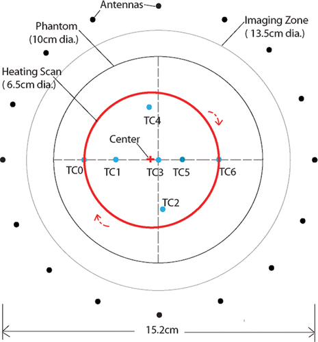
Figure 1 shows a spherical bowl ultrasound (US) transducer supported by the 3PS system (above) aimed downward into a gel phantom positioned for microwave imaging. The steering mechanism is a compact design which incorporates three computer controlled support rods that translate their vertical motion into arbitrary 3D positioning of the beam focus within the microwave imaging field of view. The US beam focus (roughly 2 cm long × 2 mm wide) is nominally oriented vertically – there is some tilt to the beam as it is steered off the central axis of the imaging plane. For these experiments the heating patterns were formed primarily in the horizontal plane for ease in comparing the microwave images with the actual temperature patterns. A more complete description of the 3PS system is available in Meaney et al. [26].

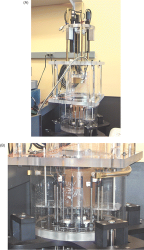
Figure 1. Photograph of the experimental set-up showing: (A) the overall experimental configuration (with the coupling liquid removed) and (B) a close-up of the imaging chamber with the gel phantom surrounded by the monopole antennae which pass through the floor of the tank and can be vertically positioned to the desired height.

The focused bowl transducer (Sonic Concepts, Woodinville, WA) was 8.4 cm in diameter with a focal length of 15 cm and had a 2 cm hole in the center. It was designed to operate at 1.5 MHz with a measured efficiency of greater than 85% which was determined by the manufacturer using an absorber-type radiation force balance to measure the acoustic power output compared with the RF power input. The coupling bath was comprised of a 65 : 35 mixture of glycerin and water and had a measured density of 1.16 g/cm³. Using published values from [27] and [28], we estimate that the speed of sound in this mixture was 1816 m/s with an attenuation coefficient of 0.53 dB/cm.

Phantom configuration

Figure 1 also shows the 10.2 cm diameter phantom used in the heating experiments with thermocouple wires protruding through its cylindrical surface. The thermocouples were implanted in the phantom during the curing process to minimize internal material perturbations. Their associated feed wires were arranged horizontally to reduce the coupling of the electromagnetic fields generated by the microwave imaging system which were predominantly oriented in the vertical direction. The gel was comprised of 500 ml of water, 4.5 g of NaCl, and 30 g of agar powder and was mixed thoroughly for 3 h with a magnetic stirring mechanism. The mixture was stabilized over a 12-h period (covered) to allow bubbles to rise to the surface and escape after which it was heated in a convection oven at 120°C for 2 h. From visual examination (and the heating experiments), the gel was found to be relatively free of air bubbles. The dielectric properties of the gel were measured at 1100 MHz to be ϵ_r = 52.7 and σ = 0.73 S/m, respectively, using an Agilent 85070E Dielectric Probe Kit in conjunction with an Agilent E5071B Network Analyzer. The acoustic and thermal properties of the gel can only be estimated at this time. From data tabulated in [24], similar agar gels were reported to have a speed of sound in the order of 1560 m/s. Corresponding estimates for the thermal conductivity range from 0.597 to 0.609 W/mK, for diffusivity from 1420 to 1560 cm²/s, and for specific heat from 3.84 to 4.03 J/gK.

Temperature measurements

For these experiments we used Omega 5TC-TT-J-30–72 thermocouples which were 0.25mm in diameter with perfluoroalkoxy (PFA) insulation and nominally produced a response time of 0.25 seconds. We used several thermocouples simultaneously connected to a National Instruments TBX-68T terminal block for continuous temperature monitoring (every 1.6 seconds) at selected sites within the phantom.

We took care to use only as many thermocouples as was necessary because the US beam did create artifacts in the temperature measurements when it passed over the sensors. We did not position any thermocouples above the imaging plane to minimize potential distortions in the power deposition. Even with care in setting the thermocouple locations, the actual positions varied by several mm. In this instance, it was helpful to have the US/thermocouple artifact as a way of locating the actual position of each sensor with respect to the US transducer steering geometry and the microwave imaging array.

Microwave data acquisition

The set of monopole antennae was configured as a circular array surrounding the phantom placed in the illumination chamber where the antenna centers (i.e. the imaging plane) were aligned with the plane of the thermocouples through computer-controlled adjustment of their vertical height relative to the floor of the imaging tank (see Figure 1). Each antenna individually broadcasts a burst of continuous wave (CW) signal (roughly 1 second) at the specified illumination frequency which is simultaneously recorded at the remaining antenna array elements. After signal transmission by one antenna, the others sequentially act as the transmitter while the remaining complement serve as receivers. The transceiver module associated with each antenna allows all channels to act as both transmitter and receiver. During reception, the detected CW signal is down-converted with a coherent reference CW signal offset by a pre-determined frequency such that the low pass filtered IF (intermediate frequency) output can be sampled by an A/D board. A detailed description of the transceiver modules can be found in Li et al. [29]. In these experiments we utilized two eight-channel, 24 bit, PXI-4472B National Instrument boards to cover the full dynamic range (130dB) without any dynamic gain control.

An initial data set was acquired without the phantom present as part of the calibration procedure [29]. Full data sets were recorded at 900 and 1100 MHz during the experiments. The data acquisition time for each frequency was 17.6 seconds making the repetition time between thermal scans 35.3 seconds. Because of the relatively long data acquisition time, some temporal averaging of the temperature induced conductivity change is expected. The calibration data were subtracted from the raw signal acquisitions during the heating procedure (in terms of both magnitude and phase) to produce calibrated measurements which were subsequently used in the reconstruction algorithm to generate images for each acquisition time point.

Image reconstruction

The microwave signal data were reconstructed into 2D multiple permittivity and conductivity images for each acquisition time using a Gauss-Newton iterative algorithm which incorporated log (variance stabilizing) transformation [30], [31]. The field solutions were computed using a hybrid of the finite and boundary element methods with a 13.5 cm diameter mesh of 3903 nodes and 7588 triangular elements having an average nodal spacing of 2.25 mm [32]. The reconstruction parameter mesh consisted of 559 nodes and 1044 elements with its perimeter aligning exactly with the field mesh [33]. The algorithm utilized a combined Levenberg-Marquardt and Tikhonov regularization [21] and applied an adjoint approach for computing the associated Jacobian matrix which produced significant computation time reductions [34]. The process completed in 10 iterations consuming a total computation time of 11 minutes on an offline Intel-based, dual-core, Xeon 2.8 GHz workstation. The reconstruction assumed a homogeneous background – in this case the coupling medium was comprised of a 65 : 35 mixture of glycerin and water with dielectric properties of ϵ_r = 48.3 and σ = 1.39 S/m, measured at 1100 MHz with a dielectric probe kit – and did not require any a priori information.

Results and discussion

We conducted three sets of phantom experiments to illustrate microwave thermal imaging in coordination with 3PS-based steerable focused ultrasound heating. For the purposes of brevity we only show representative 1100 MHz results (the 900 MHz data produced comparable images) that have been differenced with a baseline image (prior to heating) to highlight the spatial and temporal performance characteristics of the system. Actual temperatures were recorded at select locations within the imaging plane to validate the property changes. The three heating patterns included: (1) a continuously scanned 6.5 cm diameter circle, (2) a continuously scanned 240° arc of a 4.8 cm diameter circle (alternating clockwise and counter-clockwise progressions), and (3) a continuously repeated pattern of four sequentially scanned spirals (1.6 cm diameter) at different spatial locations. In each of these experiments the maximum temperature increase was less than 5°C which limited the smoothing effects from thermal conduction and allowed more complex spatial patterns in the temperature distributions to exist.

Large diameter circular scan

Figure 2 shows a diagram indicating the scan pattern for this experiment in relation to the monopole antennae and the gel phantom. The scan time for each circle was 37.6 seconds, and the RF power was turned on to a focal point intensity of 1370 W/cm² at 25 seconds and turned off at 1420 seconds (about 23 minutes later). The intensity value is an estimate based on the manufacturer's specification of the transducer efficiency in water, the measured input RF power and the surface area of the transducer.

Figure 2. Schematic diagram of the US beam steering sequence for the 6.5 cm diameter circular scan experiment.

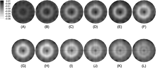
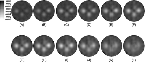
Figure 3 shows a sequence of 1100 MHz conductivity difference images for a progression of image acquisitions during heating and cooling of the phantom. The circular path of the US beam is evident as an annulus of decreasing conductivity from 143 seconds through 1391 seconds. The conductivity in the annular ring decreases evenly and nearly instantaneously after the heating commenced while the conductivity decrease in the center of the circle is less pronounced and delayed as would be expected since its temperature rise is due solely to thermal conduction from heating generated by the power deposition in the ring. Interestingly, the central conductivity decrease continues after the RF power has been turned off (at 1420 secs) while the conductivity in the ring begins to increase as the temperature subsides when no more US power is being directly deposited in that zone.

Figure 3. Sequence of 1100 MHz conductivity difference images at time points (in seconds from the start of the first microwave image acquisition) during and after heating (US power was turned on at 143 seconds and off at 1420 seconds) from the beam steering pattern shown in Figure 2: (A) 143, (B) 321, (C) 499, (D) 678, (E) 856, (F) 1034, (G) 1213, (H) 1391, (I) 1569, (J) 1748, (K) 1926, and (L) 2105 seconds, respectively. Difference images were formed by subtracting the pre-heating baseline conductivity image from the conductivity image acquired at the time points indicated.

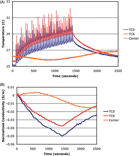
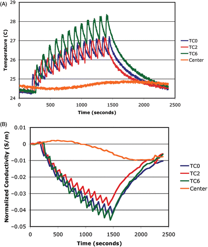
Figure 4 shows the temperatures measured by thermocouples at two locations on the circle and at the center along with spatial averages of the imaged conductivity difference at the same sites as functions of time. The averages were computed using the recovered values at the three closest conductivity estimates to the actual thermocouple site. The temperature plots show spikes at time points when the US beam passed directly over the thermocouple. The spikes for the two curves are out of phase with each other because the thermocouples were physically located 180° degrees apart along the circular heating arc. As expected, the temperatures at the two circle sites increase rapidly as the heating commences (ignoring the spike artifact) and taper off gradually, while the temperature at the center position starts rising gradually well after the RF has been turned on and continues to rise after power is shut-off. The temperatures drop off exponentially at the two circle sites after the RF is turned off. The plots of conductivity difference (Figure 4B) track the corresponding thermocouple behavior quite well. This experiment confirms that the beam can be steered in the desired pattern and that the recovered conductivity difference images are good surrogates for the overall temperature distribution. The slight temperature decrease measured at the center of the phantom during the early portion of the experiment is likely due to cooling from residual heating during initial testing of the experimental set-up prior to beginning the actual scan pattern used in this case. Interestingly, the conductivity difference images (see Figure 4B) also illustrate this behavior which is excellent confirmation of the sensitivity of the imaging system to these small changes (<0.5°C) in temperature.

Figure 4. Plots of (A) temperature and (B) average conductivity difference as a function of time at selected points in the imaging plane: thermocouples (TC) 0 and 6 reside along the path scanned by the beam focus (see Figure 2). A reference measurement is included from the center of the imaging zone.

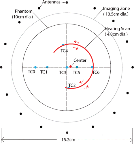
Partial circular arc heated scan

Figure 5 shows a diagram depicting the scan pattern for this experiment. The time for a single complete clockwise and counter-clockwise scan was 56 seconds (20 total scans) and the RF was turned on to a focal point intensity of 1370 W/cm² at 120 seconds and turned off at 1280 seconds (approximately 20 minutes later).

Figure 5. Schematic diagram of the US beam steering sequence for the partial circular scan experiment.

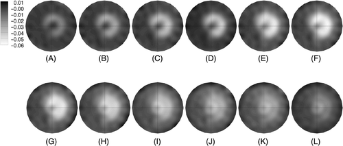
Figure 6 shows the sequence of 1100 MHz conductivity difference images for a progression of image acquisitions during heating and cooling of the phantom. The time sequence from 321 to 1213 seconds shows a C-shaped distribution of lower conductivity slowly appearing in the upper right quadrant of the field of view and becoming more pronounced in terms of lower conductivity with time. In addition, the width of the beam line gradually increases, presumably from thermal conduction outward from the line which almost fills the central area after 1213 seconds. From time 1391 to 2283 seconds, the RF power has been shut off, and the difference images show that the conductivity in the directly heated areas begins to revert back to baseline while the conductivity continues to decrease in the center (especially from times 1391 to 1926 seconds) reflecting the temperature rise.

Figure 6. Sequence of 1100 MHz conductivity difference images at time points (in seconds from the start of the first microwave image acquisition) during and after heating (US power was turned on at 120 sec and off at 1280 sec) from the beam steering pattern shown in Figure 5: (A) 321, (B) 499, (C) 678, (D) 856, (E) 1034, (F) 1213, (G) 1391, (H) 1569, (I) 1748, (J) 1926, (K) 2105, and (L) 2283 seconds, respectively. Difference images were formed by subtracting the pre-heating baseline conductivity image from the conductivity image acquired at the time points indicated.

Figure 7 shows the temperatures measured by thermocouples at three locations along the arc and at the center along with spatial averages of the imaged conductivity difference at the same sites as functions of time. For the three arc locations, temperature spikes associated with the beam passing directly over the thermocouple are present. The beam's lower terminus was very close to TC2 causing only 20 spikes, while it passed over TC6 in both the clockwise and counter-clockwise sweeps for a total of 40 spikes. Interestingly, the upper beam terminus was slightly beyond TC4 such that the clockwise and counter-clockwise sweeps over the thermocouple were very close in time subsequently creating a broader artifact than for the other two sensors. For each of these three plots, an interpolation of the lower part of each curve would be a more accurate indication of the actual temperatures, because the elevated spikes are associated primarily with the beam/thermocouple interaction. In these cases, the temperatures rise most rapidly at the start of heating and gradually taper off near the end of heating. After power is turned off, they all drop exponentially during the cooling process. The central temperature does not begin to increase until roughly 400 seconds and continues to increase gradually well after the heating has ceased, as would be expected due to conductive heat transfer.

Figure 7. Plots of (A) temperature and (B) average conductivity difference as a function of time at selected points in the imaging plane: TC2 is located at the lower terminus of the scanned heating arc, TC4 is near the upper terminus (but not on it), and TC6 is midway along the arc, respectively. A reference measurement is included from the center of the imaging zone.

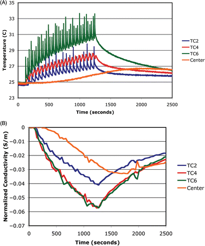
Similarly to the temperature plots, the conductivity decreased at the start of heating with some leveling off towards the end of the exposure. All three conductivity values rose in an exponential fashion after the RF had been turned off. In addition, the central conductivity values start to decrease gradually after a delay of approximately 400 seconds after the RF is turned on and continue to rise until 1752 seconds, well after the heating has ceased and very similarly in nature to the associated temperature plot. The conductivity difference traces exhibit some variations, with the most significant aberration occurring near 1900 seconds; however, the overall behavior of the curves corresponds well to the actual temperature profiles.

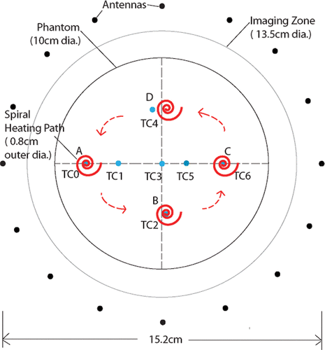
Four sequential spiral scans

Figure 8 shows a diagram depicting the scan pattern for this experiment. The beam traced a series of horizontal (within the imaging plane) spirals each centered at the locations indicated. The outer diameter of each spiral was 1.6 cm consisting of 720° of total rotation. The scan time for the first three spirals (A, B, C centered on thermocouples TC0, TC2 and TC6, respectively) was 30 seconds while that for the fourth, D, was only 12 seconds. The RF power was turned on to a focal point intensity of 910 W/cm² at 210 seconds and turned off after 12 consecutive sets of the 4 spirals (a thirteenth spiral was also scanned at A) at 1464 seconds.

Figure 8. Schematic diagram of the US beam steering sequence for the four sequential spiral scan experiment.

Figure 9 shows a sequence of 1100 MHz conductivity difference images for increasing times during and after the spiral heating sequence. The first nine images show progressively reduced conductivity spots primarily at locations A, B, and C with a much more modest conductivity decrease at the fourth location just above the center of the field of view at times 1070 through 1498 seconds. This is expected because considerably more energy is deposited at the first three locations than the last position due to the longer beam dwell time. The last three images were acquired after the heating was turned off and show the three focal conductivity decreases reverting gradually back towards their baseline values. It is interesting to note that the three primary conductivity perturbations do appear to both decrease and increase in time with a general downward trend for the first nine image times. This is due in part to the fact that the heating at each spiral occurs over 30 (first three) and 12 (last one) seconds with delays of 72 (first three) and 90 (last one) seconds, respectively, while the spirals are scanned at the other locations which allows some cooling to occur at each location.

Figure 9. Sequence of 1100 MHz conductivity difference images at time points (in seconds after the first microwave image acquisition) during and after heating (US power was turned on at 210 seconds and off at 1484 seconds) from the beam steering pattern shown in Figure 8: (A) 357, (B) 499, (C) 642, (D) 785, (E) 927, (F) 1070, (G) 1213, (H) 1355, (I) 1498, (J) 1641, (K) 1784, and (L) 1926 seconds, respectively. Difference images were formed by subtracting the pre-heating baseline conductivity image from the conductivity image acquired at the time points indicated.

Figure 10 shows the temperatures measured by thermocouples at the three spiral centers along with spatial averages of the imaged conductivity differences at the same sites as functions of time. For the three spiral locations, sharp spikes in the temperature are followed by an exponential decrease until the subsequent spike with the overall baseline temperatures increasing in time during the heating period. While a portion of each saw tooth-like segment is due to the US beam/thermocouple interaction, the time interval between heating at any one location is sufficient for some cooling to occur and be detected by the thermocouples. As would be expected, the occurrence of the spikes at the three thermocouples is out of phase since each was heated at different times during the spiral cycles. In addition, the temperature in the center of the phantom did not begin to rise until well after the heating started and only began to decrease well after the RF was turned off. Interestingly, it appears that the phantom did not completely cool down from the previous experiment because the center temperature was still decreasing during the first 500 seconds after which it started to rise again due to the heat conduction from the spiral scan sites.

Figure 10. Plots of the (A) temperature and (B) average conductivity difference as a function of time at selected points in the imaging plane: TC0 is located at the center of the first spiral scan of the beam focus, TC2 at the center of the second spiral, and TC6 at the center of the third spiral, respectively. A reference measurement is included from the center of the imaging zone.

Similarly to the temperature plots, the imaged conductivity difference values at the thermocouple sites show an overall decrease in time with a saw tooth-like pattern associated with the on and off heating characteristics of this experiment. It should be noted that the image acquisition time was not synchronized with the onset of heating at each location and that because of the relatively long data acquisition time for an individual frequency (roughly 17.6 seconds), some averaging of the actual property distributions is expected. Nonetheless, the temporal correspondence of the conductivity maps with the actual temperature data is quite good. It is also important to note that the conductivity in the center of the image did not begin to decrease until well after the RF was turned on. Interestingly, the center conductivity also exhibited a gradual increase at the start of the experiment which corresponds to the fact that the actual temperature was still decreasing as a result of residual conductive cooling from the previous experiment.

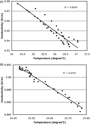
In addition, we quantitatively assessed the accuracy with which the conductivity change tracked the actual temperature for representative locations in this experiment. Figures 11A and B show plots of the conductivity versus temperature for (a) a single thermocouple location (TC0) and (b) the center of the phantom, respectively. In these graphs, data from both the heating and cooling periods were used. Conductivity linearly tracked with temperature very well. More deviation (compare Figure 11A with 11B) from the trend line occurred at TCO likely due to the fact that the measured temperatures have errors associated with the artifacts caused by the ultrasound beam when it was aimed directly at the thermocouple during the scanning process. The correlation coefficients were 0.86, 0.84, 0.80, and 0.97 for the TCO, TC2, TC6 and phantom center locations, respectively. The associated temperature accuracy (computed as an average of the temperature deviation of each data point from each trendline) was 0.18°, 0.23°, 0.35°, and 0.01°C for the TCO, TC2, TC6 and phantom center locations, respectively, indicating that the level of accuracy with which the recovered conductivity can track the actual temperature is high, even when the artifacts associated with the ultrasound beam/thermocouple interactions are taken into account.

Figure 11. Plot of the reconstructed conductivity as a function of actual temperature for the data shown in Figure 10 for (A) TC0 and (B) at the center of the phantom.

Conclusions

We have successfully integrated a scanned focused US therapy transducer for hyperthermia with a microwave imaging array for non-invasive temperature monitoring. The US beam steering primarily utilizes vertical motion of the transducer support rods which occupy minimal space and do not interfere with the microwave illumination zone. We have demonstrated that the system can scan a range of arbitrary geometries and heating patterns with concurrent thermal imaging which could be useful in various therapy settings. The phantom experimental results are encouraging in terms of capturing the overall temperature characteristics of the heated zones especially with respect to their temporal variations. They show that the gel properties do indeed vary with temperature and that the microwave imaging system is sufficiently sensitive to capture these variations. Specifically, temperature sensitivity and accuracy are better than 0.5°C and 0.35°C, respectively, in the experiments performed here. Small temperature changes of less than a degree recorded in the center of the phantom during the early stages of a heating experiment involving a particular scan pattern resulting from the cooling of residual temperature elevations in prior experiments were captured in the conductivity images. Cyclic heat-up and cool-down behavior in recorded temperatures due to spatial cycling of the US beam pattern with periods of less than 100 seconds were also evident in the imaged conductivity maps. These results suggest that the temporal and thermal resolutions of the imaging procedure are sufficient for most clinical applications.

The next step in developing and evaluating this combined therapy/monitoring system will be to apply it in animal experiments. Important advances will be needed to provide the heating from below (or side) the animal with the beam aimed upwards (or from the side) at the target tissue from within the coupling bath. The 3PS system is well suited to this configuration because the transducer support rods can be mounted to slide through hydraulic seals in the tank base (or walls) similarly to the way in which the microwave monopole antennae already move through the tank wall. In addition, it may not be physically possible to position a full circular array of antennae completely around the treated tissue. However, we have shown in recent experiments that we can recover high quality images from arrays that partially surround a target zone. Speed of data acquisition and image processing remains a challenge as well. We are currently fabricating a microwave system that will be capable of acquiring single image data sets at a rate of 20 frames/sec compared to the current system which records one image every 15 seconds. This will be a dramatic improvement in temporal resolution. The image reconstruction time will also significantly improve with further algorithm optimization and the use of parallel processing and/or field programmable gate array (FPGA) processors dedicated to the computations.

Finally, biological and/or physiological challenges to the thermal imaging approach also remain as the linearity of electrical conductivity change with temperature is expected to degrade when large elevations are sustained over time during treatments and may vary with tissue composition and/or perfusion effects that are likely to be present in vivo during thermal therapy. While we expect to be able to recover reliable electrical property maps that vary over time during a heating procedure, interpretation of these changes in terms of temperature or some other surrogate of treatment effect awaits further study.

Acknowledgement

This work was supported by NIH/NIBIB Grants RO1-EB001982 and R44- EB003666.

Declaration of interest: Dr. Meaney and Paulsen are co-founders of Microwave Imaging System Technologies, Inc. in Hanover, NH which has several patents related to microwave tomographic imaging. The authors alone are responsible for the content and writing of the paper.

References

- Valdagni R, Amichetti M. Report of long term follow-up in a randomized trial comparing radiation therapy to radiation therapy plus hyperthermia for metastatic lymph nodes in stage IV head and neck patients. Int J Radiat Oncol Biol Phys 1994; 28: 163–169
- Vernon CC, Hand JW, Field SB, Machin D, Whaley B, van der Zee J, van Putten WLJ, van Rhoon GC, van Dijk JDP, González DG, et al. Radiotherapy with or without hyperthermia in the treatment of superficial localized breast cancer: Results from five randomized controlled trials. Int J Radiat Oncol Biol Phys 1996; 35: 731–744
- Overgaard J, Gonzalez-Gonzalez D, Hulshof MCCM, Arcangeli G, Dahl O, Mella O, Bentzen SM. Randomized trial of hyperthermia as adjuvant to radiotherapy for recurrent or metastatic malignant melanoma. Lancet 1995; 345: 540–543
- Van der Zee J, Gonález D, van Rhoon GC, van Dijk JDP, van Putten WLJ, Hart AM. Comparison of radiotherapy alone with radiotherapy plus hyperthermia in locally advanced pelvic tumours: A prospective, randomized, multicentre trial. Lancet 2000; 355: 1119–1125
- Westermann AM, Jones EL, Schem B-C, van der Steen-Banasik EM, Koper P, Mella O, Uitterhoeve ALJ, de Wit R, van der Velden J, Burger C, et al. First results of triple-modality treatment combining radiotherapy, chemotherapy, and hyperthermia for the treatment of patients with stage IIB, III, and IVA cervical carcinoma. Cancer 2005; 104: 763–770
- Jones EL, Oleson JR, Prosnitz LR, Samulski TV, Vujaskovic Z, Yu D, Sanders LL, Dewhirst MW. Randomized trial of hyperthermia and radiation for superficial tumors. J Clin Oncol 2005; 23: 3079–3085
- Paulsen KD, Hartov A, Meaney PM. Matching the energy source to the clinical need. The International Society for Optical Engineering, TP Ryan. SPIE Optical Engineering Press, San Jose, CA 2000; 485–515
- Sreenivasa G, Gellermann J, Rau B, Nadobny J, Schlag P, Deuflhard P, Felix R, Wust P. Clinical use of the hyperthermia treatment planning system HyperPlan to predict effectiveness and toxicity. Int J Radiat Oncol Biol Phys 2003; 55: 407–419
- Deuflhard P, Seebass M, Stalling D, Beck R, Hege H-C. Hyperthermia treatment planning in clinical cancer therapy. Modelling, simulation, and visualization. IMACS World Congress, Jackson Hole, Wyoming. 1997; SC 97–26
- Van de Kamer JB, De Leeuw AAC, Hornsleth SN, Kroeze H, Kotte ANTJ, Lagendijk JJW. Development of a regional hyperthermia treatment planning system. Int J Hyperthermia 2001; 17: 207–220
- Gellermann J, Wust P, Stalling D, Seebass M, Nadobny J, Beck R, Hege H, Deuflhard P, Felix R. Clinical evaluation and verification of the hyperthermia treatment planning system hyperplan. Int J Radiat Oncol Biol Phys 2000; 47: 1145–1156
- Vigen KK, Jarrard J, Rieke V, Frisoli J, Daniel BL, Pauly KB. In vivo porcine liver radiofrequency ablation with simultaneous MR temperature imaging. J Mag Res Imag 2006; 23: 578–584
- Arora D, Cooley D, Perry T, Guo J, Richardson A, Moellmer J, Hadley R, Parker D, Skliar M, Roemer RB. MR thermometry-based feedback control of efficacy and safety in minimum-time thermal therapies: Phantom and in-vivo evaluations. Int J Hyperthermia 2006; 22: 29–42
- Jolesz FA, Hynynen K, McDannold N, Tempany C. Imaging-controlled focused ultrasound ablation: A noninvasive image-guided surgery. Mag Res Imag Clin North America 2005; 13: 545–560
- Peller M, Kurze V, Loeffler R, Pahernik S, Dellian M, Goetz AE, Issels R, Reiser M. Hyperthermia induces T1 relaxation and blood flow changes in tumors. A MRI thermometry study in vivo. J Mag Res Imag 2003; 21: 545–551
- Craciunescu OI, Das SK, McCauley RL, MacFall JR, Samulski TV. 3D numerical reconstruction of the hyperthermia induced temperature distribution in human sarcomas using DE-MRI measured tissue perfusion: Validation against non-invasive MR temperature measurements. Int J Hyperthermia 2001; 17: 221–239
- Quesson B, de Zwart JA, Moonen CT. Magnetic resonance temperature imaging for guidance of thermotherapy. J Mag Res Imag 2000; 12: 525–533
- Clegg ST, Das SK, Zhang Y, Macfall J, Fullar E, Samulski TV. Verification of a hyperthermia model method using MR thermometry. Int J Hyperthermia 1995; 11: 409–424
- Hynynen K, Pomeroy O, Smith DN, Huber PE, McDannold NJ, Kettenbach J, Baum J, Singer S, Jolesz FA. MR imaging guided focused ultrasound surgery of fibroadenomas in the breast: A feasibility study. Radiol 2001; 219: 176–185
- Jacobsen S, Stauffer PR. Multifrequency radiometric determination of temperature profiles in a lossy homogeneous phantom using a dual-mode antenna with integral water bolus. IEEE Trans Microwave Theory Tech 2002; 50: 1737–1746
- Meaney PM, Paulsen KD, Fanning MW, Li D, Fang Q. Image accuracy improvements in microwave tomographic thermometry: Phantom experience. Int J Hyperthermia 2003; 19: 534–550
- Meaney PM, Fanning MW, Paulsen KD, Li D, Pendergrass SA, Fang Q, Moodie KL. Microwave thermal imaging: Initial in vivo experience with a single heating zone. Int J Hyperthermia 2003; 19: 617–641
- Siep R, Ebbini ES. Noninvasive estimation of tissue temperature response of heating fields using diagnostic ultrasound. IEEE Trans Biomed Eng 1995; 42: 828–839
- Duck FA. Physical properties of tissues: A comprehensive reference book. Academic Press, London 1990; 121–123, 173
- Miller NR, Bamber JC, Meaney PM. Fundamental limitations of non-invasive temperature imaging by means of ultrasound echo strain imaging. Ultrasound Med Biol 2002; 28: 1319–1333
- Meaney PM, Raynolds T, Potwin L, Paulsen KD. 3-Point support mechanical steering system forhigh intensity focused ultrasound. Phys Med Biol 2007; 52: 3045–3056
- Saggin R, Coupland JN. Concentration measurement by acoustic reflectance. J Food Sci 2001; 66: 681–685
- Zorebski E, Zorebski M, Gepert M. Ultrasonic absorption measurements by means of a megahertz-range measuring set. Fifth Winter School on Wave and Quantum Acoustics, J Bodzenta, M Dzida, T Pustelny. J Phys IV. 2006; 137: 231–235
- Li D, Meaney PM, Raynolds T, Pendergrass SA, Fanning MW, Paulsen KD. A parallel-detection microwave spectroscopy system for breast imaging. Rev Sci Instrum 2004; 75: 2305–2313
- Meaney PM, Paulsen KD, Pogue BW, Miga MI. Microwave image reconstruction utilizing logmagnitude and unwrapped phase to improve high-contrast object recovery. IEEE Trans Med Imag 2001; 20: 104–116
- Meaney PM, Fang Q, Rubaek T, Demidenko E, Paulsen KD. Log transformation benefits parameter estimation in microwave tomographic imaging. Med Phys 2007; 34: 2014–2023
- Meaney PM, Paulsen KD, Chang JT. Near-field microwave imaging of biologically based materials using a monopole transceiver system. IEEE Trans Microwave Theory Tech 1998; 46: 31–45
- Paulsen KD, Meaney PM, Moskowitz MJ, Sullivan JM, Jr. A dual mesh scheme for finite element based reconstruction algorithms. IEEE Trans Med Imag 1995; 14: 504–514
- Fang Q, Meaney PM, Geimer SD, Streltsov AV, Paulsen KD. Microwave image reconstruction from 3D fields coupled to 2D parameter estimation. IEEE Trans Med Imag 2004; 23: 475–484