Inverse method for quantitative characterisation of breast tumours from surface temperature data

Abstract

Purpose: We introduce a computational method to simultaneously estimate size, location and blood perfusion of the cancerous breast lesion from the surface temperature data.

Methods: A 2D computational phantom of axisymmetric tumorous breast with six tissue layers, epidermis, papillary dermis, reticular dermis, fat, gland, muscle layer and spherical tumour was used to generate surface temperature distribution and thereby estimate tumour characteristics iteratively using an inverse algorithm based on Levenberg–Marquardt method. In addition to the steady state temperature data, we modified and expanded the inverse algorithm to include transient data that can be captured by dynamic infra-red imaging. Several test cases were considered for the transient analysis, where the depth, radii and blood perfusion of tumour were varied from 11 to 30 mm, 7 to 11 mm and 0.003 to 0.01 1/s, respectively.

Results: Similar steady state temperature profile for different tumours makes it impossible to simultaneously estimate blood perfusion, size and location of tumour using steady state data alone. This becomes possible when transient data are used along with steady state data. For the cases discussed here, the estimates have errors below 1% for tumours with depths less than 20 mm, but for deeper tumours (25 mm) errors can be more than 10%.

Conclusions: Combination of transient data and steady state data makes it possible to simultaneously estimate tumour size, location and blood perfusion. Blood perfusion is an indicator of the growth rate of the tumour and therefore its evaluation can possibly lead to the assessment of tumour malignancy.

Keywords:

• Breast cancer
• thermography
• inverse methods
• Levenberg–Marquardt method
• quantitative tumour characterization

Introduction

Early detection of breast cancer is currently the most effective way to address the disease. Various test methods, such as X-ray mammography, biopsy, ultrasound, magnetic resonance imaging (MRI) and infra-red (IR) thermography have been used to detect breast cancer [1,2].

IR thermography has been increasingly used to complement other imaging modalities for breast cancer detection [2,3]. It is non-invasive in nature and relatively less expensive than some other diagnostic modalities, such as MRI. Malignant tumours generate excess heat because of increased metabolic heat generation and they also require an increased supply of blood to support growth of cancerous cells, generally increasing local temperatures which can be detected with thermography [2,4]. A longitudinal study conducted by Gautherie and Gros [5] determined that earlier detection of cancer was possible when thermography was combined with other techniques.

Gautherie [6] also noted that tumours with faster growth rate had higher probability of dissemination as well as higher metabolic heat generation rate, and established a relationship between metabolic heat generation and cancer growth rate. Subsequently, others have related high micro vessel density with higher risk of metastasis [7–10]. It has been proposed that an estimation of the metabolic activity of the tumour from surface temperature measurements can provide a measure of the malignancy of the tumour. This is potentially advantageous, and reinforces the relevance of IR thermography in clinical settings, particularly in resource-poor or underserved regions of world. The relative portability and low cost of IR equipment can promote enhanced detection and clinical management of breast cancer to address current disparities in clinical care.

High vascularisation necessary to support accelerated malignant cell growth can be quantified in terms of the local blood perfusion rate, when this can be accurately measured. Therefore both increased metabolic activity (heat generation) and increased blood perfusion rate can serve as markers of malignancy. Prior studies on melanoma (clinical and computational modelling [11]) and breast cancer (computational modelling [12]) suggest that the influence of blood perfusion on the thermal signature of the cancerous lesion is more pronounced than metabolic heat generation rate. Based on the sensitivity analysis, Çetingül and Herman [11] and Cheng and Herman [13] concluded that surface temperature is most sensitive to blood perfusion rate and tissue layer thickness.

To date, thermography has been a largely qualitative technique, and diagnosis was based on qualitative criteria such as asymmetry, hyperthermic patterns and abnormal vascular patterns [2]. Quantitative information is typically extracted by comparing temperature increase at two separate locations of tissue arbitrarily selected by the operator. Currently lacking are additional quantitative components to enhance the robustness of interpretation of thermal images. Extracting detailed parameters (location, size, perfusion) of an object, such as tumour, from observable surface temperature data fits within the group of “inverse problems” that occur in various fields including medicine [14–22].

We use the Pennes’s bioheat transfer equation [23] to model heat transfer processes inside human tissue, and compute surface temperature signatures which serve as input data for the inverse reconstruction algorithm. Then, based on the surface temperature profile, we estimate tumour parameters. During the past few years, several research teams [14–20] attempted to solve the inverse problem for breast cancer. Mital and Pidaparti [14] simultaneously estimated size, location and metabolic heat generation, and used artificial neural network (ANN) and genetic algorithm (GA) methods on a multilayer, 2D model. Bezerra et al. [16] estimated thermal conductivity and blood perfusion rate using the Sequential Quadratic Programming method. They used a 3D surrogate geometry based on external breast prosthesis. Both these researchers, Mitra and Balaji [15] and Bezerra et al. [16], used a correlation for their analysis that related the diameter of the tumour with the metabolic heat generation rate. According to this correlation, larger tumours have higher metabolic heat generation rate. However, Gautherie [6] observed that the metabolic heat generation rate was cancer-specific and case-specific and it was constant during tumour evolution. Based on his work, it can be concluded that the metabolic heat generation rate might not always be entirely dependent on the size of the tumour. Therefore, there is a need to relax this assumption inherent in the correlation used by Mitra and Balaji [15] and Bezerra et al. [16].

Mitra and Balaji [15] used the ANN method on a single tissue, 3D hemispherical model to simultaneously estimate size, location and metabolic heat generation of the lesion. It should be noted that they have used steady state data for their analysis. It will be shown in the present work that it is difficult to simultaneously estimate three tumour parameters (dimensions, location, metabolic heat generation rate or blood perfusion rate) with accuracy and uniquely, based on the steady state data alone. Das and Mishra [18,19] estimated the size and location of tumour in a 2D rectangular domain, using the GA and curve fitting method. They considered breast as a uniform tissue instead of a multilayer structure. In 2015, Das and Mishra [20] extended their analysis to 3D hemispherical domain and used curve fitting method. All these researchers have based their analysis on steady state temperature data.

Based on the literature survey conducted, a need for an inverse reconstruction method exists that will allow us to simultaneously and uniquely estimate size, location and blood perfusion rate, a measure for the metabolic activity of the tumour based, on the surface temperature signature. In the present work we used, the Levenberg–Marquardt (LM) method [24] to uniquely and simultaneously estimate the above-mentioned parameters. We found that for this inverse analysis the steady state surface temperature was not sufficient to yield a unique solution, therefore, we added the transient data set to our inverse reconstruction algorithm. Transient data were generated by applying a cooling load and then recording the temperature as the tissue recovered [13,25]. It should be noted here that transient analysis has been used before [26,27] for the inverse analysis, however it was limited to the estimation of the blood perfusion rate only. Kleinman and Roemer [28] also used the transient analysis on a one-dimensional model to estimate the temperature distribution and blood perfusion rate beneath the surface based on surface temperature data. Furthermore, transient analysis was also used by Bhowmik and Repaka [29] to estimate the geometric and thermophysical properties, but for melanoma. Although this looks similar to our work there are major dissimilarities, among other things we have given an explanation for the need of transient analysis, have used initial guesses far away from the exact parameters, used a different optimisation algorithm and have smaller computational time. Blood perfusion rate is an indicator of the increased cell activity in the tissue, which can be potentially related to the stage of the tumour [6]. Thus, the transient version of the inverse method has a potential to estimate the stage of the tumour by estimating blood perfusion from the surface temperature signature.

We have developed a model that combines several tissue layers, with their thermophysical properties, incorporates transient data and estimates blood perfusion along with depth and size of tumour. An inverse reconstruction method, based on LM algorithm, to characterise a tumour based on skin surface temperature was tested using computational methods. First, location and size were estimated using steady state data and then an attempt was made to simultaneously estimate third parameter, blood perfusion rate along with the other parameters. Finally, transient data were used, along with steady state data, to simultaneously estimate all three parameters. Use of transient temperature or response in combination with the steady state aids estimation of parameters, thereby resolving issues encountered with uniqueness of reconstruction based on steady state data alone.

Methods

The inverse reconstruction of tumour parameters based on surface temperature data involves several steps. In this study, we use a computational phantom of the breast with the tumour to generate the surface temperature data for the testing of the reconstruction algorithm. In a clinical implementation, these surface temperature data would be acquired by IR imaging. The advantage of using a computational phantom in the initial phase of software development, testing and validation of the inverse reconstruction method is that the exact parameters of the tumour are known. This allows easy validation of the inverse reconstruction accuracy. The computational phantom also allows the flexibility to vary tumour properties in parametric studies. Once the inverse reconstruction method is extensively tested and validated, measurement data are used. We describe the mathematical model used to generate the computational phantom, as well as to solve the direct problem in Section “Mathematical model”. The direct problem involves the calculation of the surface temperature distribution for a given set of system parameters during the iterative inverse reconstruction process. For solving the direct problem, the commercial software COMSOL Multiphysics v 4.3 (2013) [30] was used. The LM method was used to estimate the unknown tumour parameters using successive iterations and it is described in Section “Input data for the inverse problem: computational phantom”.

Mathematical model

The schematic of the investigated geometry is displayed in Figure 1. The breast shape can vary, and in this study it is modelled as a hemisphere without loss of generality. In clinical applications, the actual shape can be measured by a 3D imager, such as the Kinect. We consider a single tumour, which is spherical in shape and is located at the axis of the hemisphere. Other shapes, such as elliptical, can also be used, which would introduce additional unknowns to be determined in the inverse reconstruction. By selecting the axially symmetrical two-dimensional (2D) problem in this analysis, the computational effort is kept reasonable in the initial testing stage of the reconstruction algorithm. Also, the interpretation of the results is more intuitive and algorithm progress is easier to track for the two dimensional case. Our previous study shows that the thermal signature of the tumour on the skin surface will be very similar for off axis locations [12]. The approach can easily be generalised to a three-dimensional (3D) problem, such as those discussed by Chanmugam et al. [12], at a later stage and this would require improvements in the meshing of the direct problem. Furthermore, it is assumed in the model that the thermophysical properties of the tissue and tumour are known.

Figure 1. Schematic of the biophysical situation: breast cross section, tumour, tissue layers and the thermal boundary conditions.

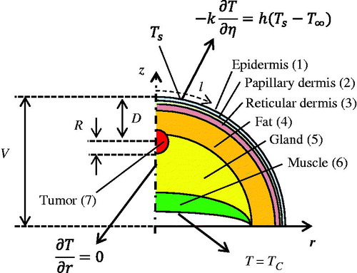
The overall goal of the inverse reconstruction is to non-invasively measure key tumour parameters, the depth and size of the tumour. Since the blood perfusion rate can be related to malignancy, we add the blood perfusion as the third parameter in our analysis. The inverse problem is solved for two cases, the first deals with steady state analysis, while the second case deals with a transient situation. For steady state, we reconstruct two unknown tumour parameters, the depth of the tumour measured from the skin surface (D) and the radius of the tumour (R) (Figure 1). In transient analysis, we reconstruct a third unknown, the blood perfusion rate (ω_b).

Human breast tissue in this analysis comprised six layers: epidermis, papillary dermis, reticular dermis, fat, gland and muscle as well as the tumour, the seventh region, as indicated in Figure 1. The Pennes bioheat equation [23] was used to model heat transfer in the layers of the breast and in the tumour as (1)

In Equation (1)(1) , ρ_b, c_b, T_b and ω_b,n represent the density and specific heat of blood, the arterial blood temperature and the blood perfusion rate of the tissue layer n, respectively. ρ_n, c_n, T_n, k_n and Q_n, are the corresponding tissue properties: density, specific heat, temperature, thermal conductivity and metabolic heat generation. The thermophysical properties for the seven tissue types are summarised in Table 1 along with their thicknesses (th_n), based on data reported by Çetingül and Herman [25], Ng and Sudharsan [31], Amri et al. [32] and Jiang et al. [33]. Density (ρ_b) and specific heat (c_b) for blood were 1060 kg/m³ and 3770 J/(kg K), respectively [25]. The radius of the hemi-spherical breast V was taken to be 72 mm [31] (Figure 1). Blood perfusion rate and metabolic heat generation rate were tumour-specific and also depend on the stage of the tumour. One of the plausible set of values is given in Table 1.

Table 1. Thermophysical properties of the tissue layers in Equation (1).

		Thickness	Thermal conductivity	Density	Heat capacity	Blood perfusion rate	Metabolic heat generation
		th, mm	k, W/(m.K)	ρ, kg/m^3	c, J/(kg.K)	ωb, 10^−4 m^3/s/m^3	Q, W/m^3
1	Epidermis [25]	0.1	0.235	1200	3589	0	0
2	Papillary dermis [25]	0.7	0.445	1200	3300	2	368.1
3	Reticular dermis [25]	0.8	0.445	1200	3300	13	368.1
4	Fat	5 [31]	0.21 [31]	930 [32]	2674 [25]	1.8 [31,33]	400 [31]
5	Gland	43.4 [31]	0.48 [31,32]	1050 [32]	3770 [32]	5.4 [31,33]	700 [31]
6	Muscle	15 [31]	0.48 [31]	1100 [32]	3800 [25]	8.1 [31,33]	700 [31]
7	Tumor	–	0.48 [31,32]	1050 [32]	3770 [32]	108 [31,33]	5000 [31]

The system of seven coupled partial differential equations described by Equation (1)(1) is solved for the following set of thermal boundary conditions.

Heat flux continuity and the temperature continuity at the interfaces of two tissue layers: (2) (3) (4) (5) where ξ is the direction perpendicular to the interface between the layers, k_adj and T_adj  are the thermal conductivity and temperature of the tissue layer adjacent to the tumour. The inner portion of the muscle layer, the region of the breast which touches the chest wall, is assumed to be at the core body temperature. (6)

The skin surface is exposed to ambient air during the exam, which leads to loss of heat to the atmosphere, described by the convective boundary condition as (7)

h = 10 Wm⁻²K⁻¹, k. = 0.235 Wm⁻¹K⁻¹, T_∞ = 21 °C where h is the convective heat transfer coefficient, k₁ is the thermal conductivity of the epidermis, the outermost tissue layer, T_1,s is the temperature of the epidermis at the skin surface interfacing the ambient and η is the direction perpendicular to the skin surface.

DynamicR imaging involves cooling of the skin surface and analysis of the transient thermal response to the excitation. Initially the skin surface is at steady state under ambient conditions. It is cooled by maintaining the surface at 14 °C for time t_c. This is modelled by using constant temperature boundary condition. (8)

The cooling in our analysis is applied for the duration of t_c= 60 s [13]. Subsequently the surface is again exposed to the ambient conditions in the exam room and hence the convective boundary condition (Equation (7)(7) ) is applied on the surface. This reheating process following the exposure to cooling is called the thermal recovery. Surface temperature data in this study are computed or recorded till 1000 s during the thermal recovery process.

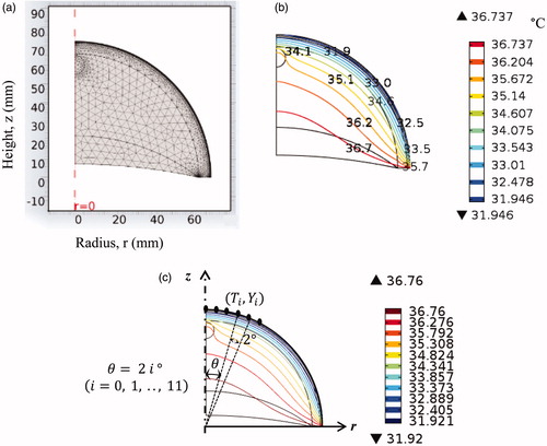
The system of seven partial differential equations [1(1) ] is solved, subject to boundary conditions (2–8) using the commercial software COMSOL Multiphysics v 4.3 (2013) [30]. A MATLAB code was developed for solving the inverse problem. While solving the inverse problem in MATLAB, COMSOL was accessed to compute temperature distributions for a given set of input parameters updated by the inverse reconstruction algorithm. For the purpose of communication and control of COMSOL by means of MATLAB, the LiveLink for MATLAB was used. The PC computer system used to run the present model was equipped with an Intel core i-7 processor, with 3.6 GHz frequency and 8 GB RAM. A typical mesh generated for the computational domain contains 8000 elements (Figure 2(a)). It takes about 6 s to solve the set of equations for steady state analysis and about 16 s for the transient analysis. Mesh sensitivity analysis was carried out to ensure that the change in temperature, due to further refinement of the mesh, was less than 0.1%. The choice of the time step was governed by two factors, computational speed and accuracy. A smaller time step increases the accuracy, but it also leads to increase in computational time. For the present case, a time step of 2 s was taken as the temperature change was less than 0.1% after decreasing the time step. The steady state temperature distribution in the cancerous breast for the conditions described by Equations (1–8), obtained using COMSOL, is shown in Figure 2(b).

Figure 2. (a) Computational mesh, (b) computed temperature distribution in the cancerous breast and (c) coordinate system and surface data points used for the inverse reconstruction.

Input data for the inverse problem: computational phantom

Input data for the inverse reconstruction algorithm are generated using the computational phantom in this study. In a clinical application computed surface temperature data (from the computational phantom) are replaced by measurement data obtained by means of IR imaging. In the computational phantom, the tumour is modelled in COMSOL for the exact set of tumour parameters R_e, D_e and ω_be. The exact set of tumour parameters for the steady state analysis (Figure 1) is stored in the vector (9)

The transient analysis accounts for an additional unknown parameter ω_b; therefore, the exact set of parameters for the transient case becomes (10)

Computed surface temperature data, obtained solving the mathematical model described by Equations (1–8) for tumour parameters from Equations (9(9) and 10(10) ), at I = 12 points on the surface, corresponding to 12 angular locations (Figure 2(c)). (11)

served as input values for the inverse reconstruction algorithm. Steady state temperature data computed using the COMSOL model are stored in the input vector Y_ss as (12) where T(θ_I=2i°) represents the surface temperature at the polar angle 2i° (Figure 2(c)).

The number of input data points in Equation (12)(12) was kept low, as a large number of data points would significantly increase computational effort and require advanced computational resources. The selected number of data points was determined by trial and error and was guided by the required accuracy for the selected application. If necessary, the number of data points in a particular application can be increased to improve reconstruction accuracy. Furthermore, the data points were distributed in the region where the temperature increase caused by the presence of the tumour is most pronounced, corresponding to the strongest measurement signal in a clinical application. In this study, they were not distributed throughout the entire circumference, rather they were concentrated within a limited region (0–22° angle) relative to the z axis (Figure 2(c)).

For the transient analysis, surface temperature data as a function of time are also collected during the thermal recovery phase at times t_j = 200 s, 400 s, 500 s, 600 s, 700 s, 800 s, 1000 s. Only one surface point is considered to describe the time dependence of temperature, in order to strike a balance between the computational cost and accuracy. The selected point is located on the skin surface directly above the tumour (θ₀=0^o), and this is the point that records the maximum temperature rise [12]. In the present work, only a single point is taken to record the transient temperature. This was sufficient to get convergence for the transient case. Adding additional data points was increasing the size of the matrix, for each data point the rank of the matrix was increasing by 7, and therefore this was taxing on the computational resources. Furthermore there were problems with convergence after adding additional data points so we avoided adding additional points.

The vector containing the surface temperatures for the transient case consists of the Y_ss, as described by Equation (12)(12) , followed by the transient data (13) where T(θ₀,t_j) represents the temperature data during thermal recovery at time t_j. The dimension of Y_tr is 19 × 1.

In clinical applications, the measured steady state or time dependent temperature will be acquired by static or dynamic IR imaging of the breast surface temperature. Typical thermal signatures were analysed computationally by Chanmugam et al. [12]. They showed that the temperature rise can be more than 1 °C for shallow and big tumours. For smaller and deeper tumours the temperature rise is low, but for the majority of the cases analysed by the authors it was more than 0.1 °C. These results suggest that modern, miniature, low-cost IR imagers are suitable for clinical diagnostic applications. The IR imager can be combined with a 3D imager, such as the Microsoft Kinect. As shown by Cheng [34], mapping 2D temperature data onto a 3D surface mesh generated by Kinect increases measurement accuracy and should be considered for clinical implementation. The geometry of the breast is not hemi-spherical and the COMSOL model can be adjusted to accommodate the exact shape when data are available.

Inverse problem: overview

In this section, we provide a general overview and rationale of the inverse reconstruction method used in our study, whereas details of the mathematical formulations of the inverse reconstruction method are introduced in Section “Inverse algorithm”. As mentioned Section “Introduction”, the problem of extracting the model parameters (tumour location, dimensions and tumour properties R, D and ω_b, E_ss or E_tr) from the observable data (measured or computed temperature distributions, Yss or Y_tr in the present study) is known as the inverse problem, and its application in heat transfer is known as the inverse heat transfer problem (IHTP). The measured or computed surface temperature distributions Yss or Y_tr (Equations (12)(12) and (13)(13) ) as well as the initial guesses of the model parameters R, D and ω_b (their exact values are to be determined by inverse reconstruction) provide the input data.

IHTP problems are very sensitive to the changes in the input data to the model and therefore are classified as ill-posed problems [24]. To overcome the ill-posedness of the problem, regularisation methods and other least square minimisation methods are used. In the current work, the LM method is implemented. In the LM method, the difference between experimental and calculated data is expressed in the form of the sum of squares S. The geometrical and thermophysical characteristics of the tumour, such as size, location and blood perfusion rate, R, D and ω_b, are adjusted iteratively, and the computed surface temperature response is compared to the measured or computed (using the phantom, Sections “Mathematical model” and “Input data for the inverse problem: computational phantom”) temperature data to minimise S. In order to counter the ill-posed nature of the problem, the LM method uses a damping factor.

The LM method iteratively solves for the tumour parameters R, D and ω_b and computes surface temperature distributions for each iteration. The iterative process continues until the difference between measured and computed surface temperatures S falls below a certain value and satisfies the stopping criterion.

Inverse algorithm

The algorithm used to solve the inverse problem is illustrated in Figures 3 and 4. The flowchart of the general algorithm is displayed in Figure 3, and details of the LM regularisation portion of the algorithm are provided in Figure 4. Each block of the algorithm is identified by a letter and the blocks are referred to by figure number and letter in the text. For example, Figure 3(a) refers to block (a) in Figure 3. It should be noted that the variables for steady state and transient state, though they have the same generic form, differ due to the presence of the additional parameter ω_b and additional transient data. These differences are described in the text and steady state and transient variables are referred to by their generic form, whenever admissible. For example, in Figures 3 and 4 only the generic forms of these variables are used.

Figure 3. Flowchart of the inverse reconstruction algorithm.

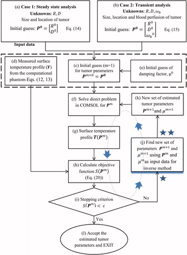
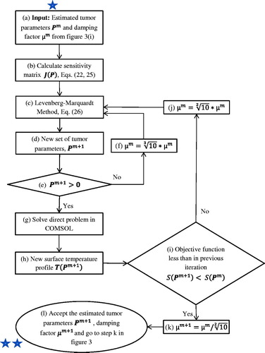
Figure 4. Flowchart describing block (j) in Figure 3.

Input data, initial guesses and process variables

The algorithm begins with an initial guess for the set of unknown parameters R, D and ω_b stored in the vector P⁰ (Figure 3(c)) as (14) (15)

The algorithm proceeds from the initial guesses to improved estimates of unknown parameters iteratively, using LM method. The set of unknown parameters at the m^th iteration is represented by the vector P^m as (16) (17)

The surface temperatures corresponding to the set of parameters P^m for the steady state analysis are stored in the vector T(P^m)as (18)

In transient analysis, T(P^m) also contains surface temperature data obtained during the thermal recovery phase corresponding to θ=0° at different times t_j (j = 1, 2, …. k), similar to the vector Y_tr described in Section “Input data for the inverse problem: computational phantom”. T(P^m) is described as (19)

The measured temperature Y, discussed in Section “Input data for the inverse problem: computational phantom” (Equations 12(12) and 13(13) ), is the second set of input data required by the algorithm (Figure 3(d)). The third input parameter used by the algorithm is the damping factor μ⁰(Figure 3(e)). The value of μ⁰ is taken to be μ⁰= 0.1 for the steady state analysis with two unknowns and the initial guess is μ⁰= 0.01 for transient analysis and the steady state analysis with three unknowns. The parameter μ⁰ is used in the LM method and it is analogous to the relaxation factor. The role of μ⁰ is explained in more detail in Section “Improving the estimates: LM algorithm”.

The commercial finite element code COMSOL is used to solve the direct problem (Figure 3(f)) of evaluating the surface temperature profile T(P^m) (Figure 3(g)) for each iteration m.

Main algorithm

The goal of the iterative procedure is to let T→Y and therefore P^m→E. To this end, we define the objective function S(P^m) (Figure 3(h)), the sum of squared errors, as [24] (20)

S(P^m) is a measure of the difference between the measured/computed temperature profile Y and the one obtained during the inverse reconstruction process based on iteratively defined tumour parameters, T(P^m) (Figure 3(g)). The form of the vectors T(P) and Y(P) is defined by Equations (12)(12) , (16)(16) and (18)(18) for the steady state analysis and Equations (13)(13) , (17)(17) and (19)(19) for the transient analysis. The set of tumour parameters P^m is accepted as the final estimate if the objective function, S(P), falls below a pre-defined value ɛ as (21)

Equation (21)(21) is referred to as the stopping criterion (Figure 3(i)), and once it is met the algorithm stops (Figure 3(l)) with the accepted set of tumour parameters P^m.

If the stopping criterion is not met, the set of parameters P^m is fed into the inverse method along with the current damping factor μ^m (Figures 3(j) and 4(a)) to find the next estimate of the unknown parameters P^m+1 and damping factor μ^m+1 (Figure 3(k)). The next estimate (m + 1) is fed into the direct problem (Figure 3(k,f)). This iterative cycle continues until the stopping criterion is met and the set of parameters hence obtained is accepted as the final estimate (Figure 3(l)).

Improving the estimates: LM algorithm

The details of the algorithm used in the “inverse method” part of Figure 3(j) are illustrated in Figure 4. The objective of this part, the LM algorithm, is to take a set of tumour parameters P^m, either the initial guess or the improved values determined through the iterative process, as input (Figure 4(a)) and compute an improved estimate of tumour parameters P^m+1 as the output (Figure 4(l)).

Based on the input parameters P^m and T(P^m), the sensitivity matrix J(P^m) is calculated first (Figure 4(b)). The sensitivity matrix accounts for the variation of surface temperature in response to the change of the tumour parameters R, D and _ωb. For the steady state analysis the sensitivity matrix is defined as (22) where I is the total number of temperature measurements on the surface (12 in this study). In the sensitivity matrix, an element located at i^th column and j^th row describes the variation of surface temperature at j^th location with respect to parameter P_i. J_ss(P_m) in Equation (22)(22) is a 12 × 2 matrix, as we have two unknown parameters, R and D, and 12 measurement points.

Individual elements of the sensitivity matrix are calculated using the approximation (23)

The term P_+j in Equation (23)(23) is defined as

for the steady state analysis.

ΔP in Equation (23)(23) is a pre-defined, fixed increment for the tumour parameters R and D, ΔP = [0.2 mm, 0.2 mm]. The sensitivity matrix for the transient case is (24) where and for times t_j during thermal recovery t: {200 s, 400 s, 500 s, 600 s, 700 s, 800 s, 1000 s} .

Elements of the sensitivity matrix for the transient situation are also determined using Equation (23)(23) . For the transient case, the term P_+j in Equation (23)(23) is defined as (25)

The dimensions of the sensitivity matrix J_ss(P^m) are 3 × 19, larger than for steady state (Equation (22)(22) ), because of the additional unknown parameter ω_b and the difference in the expressions for T(P) (Equations (18)(18) and (20)(20) ). Since the increment vector ΔP for the transient case has an additional element accounting for ω_b, it takes the form ΔP = [0.2 mm, 0.2 mm, 0.0001 ml/sec/ml]. Different values of ΔP were tried and tested. The value used in the present work was selected by trial and error and delivered the best results, in terms of convergence and computational time, and therefore it was chosen.

After determining the sensitivity matrix, the LM method (Figure 4(c)) is used to calculate the next set of parameters P^m+1 is (Figure 4(d)). (26) where Ω^m= diag ( J^m)^TJ^m.

In Equation (26)(26) , m represents the current iteration step and μ^m is the corresponding damping factor. As the damping factor is increased, the algorithm becomes more stable at the expense of speed. The damping factor controls the difference between P^m and probable P^m+1; the larger μ^m is, the smaller will be the difference between tumour parameters in successive iterations, thereby making the algorithm slower. Furthermore, the term “diag” in Equation (26)(26) refers to a diagonal matrix comprised of the diagonal elements of the corresponding matrix.

The next set of parameters P^m+1 hence obtained is checked (Figure 4(e)): if one of the parameters is negative, they are discarded and the LM method is used again (Figure 4(c,d)) after increasing damping factor μ by a factor of (Figure 4(f)). The resulting set of parameters is checked again (Figure 4(e)) and this cycle continues until the algorithm yields a set of realistic (positive) parameters. Based on the new set of parameters P^m+1, the direct problem is solved (Figure 4(g,h)) and the corresponding objective function S(P^m+1) (Equation (22)(22) ) is calculated. This new parameter P^m+1 is accepted only when the corresponding objective function S(P^m+1) is less than the one associated with the previous input parameter set P^m (Figure 4(i)) (27)

If this condition is met, the damping factor is decreased by a factor of (Figure 4(k)) and the new set of parameters P^m+1 is accepted (Figure 4(l)). On the other hand, if the objective function is larger, the set of parameters is discarded and the damping factor is increased by a factor of (Figure 4(j)). Then LM method is used again to obtain a new set of parameters (Figure 4(c)). This process continues until a set of parameters is obtained which is better than the set of parameters from the previous iteration, in terms of objective function (Equation (27)(27) ).

Results and discussion

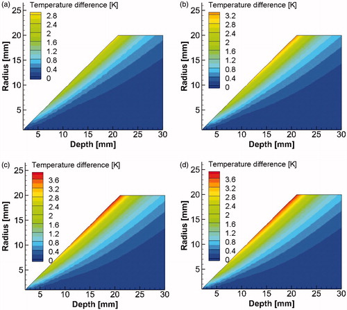
In Section “Steady state analysis with two unknowns (R and D)”, we introduce inverse reconstruction results for steady state analysis. We demonstrate that the steady state analysis has some inherent limitations, and we analyse these in Section “Limitations of the steady state analysis”. Finally, in Section “Solution: transient analysis”, we show how to overcome these limitations by including transient temperature data in the inverse reconstruction algorithm. In the present study, only those tumours were considered which were capable of giving a detectable temperature rise on the skin surface. Figure 5 shows the temperature rise, at skin surface directly above the tumour, for different combinations of radius R, depth D and blood perfusion ω_b.

Figure 5. Temperature rise ΔT at a point directly above the tumour corresponding to θ₀=0^o as a function of tumour radius R and depth D for blood perfusion values (a) ω_b=  0.003 m³/s/m^3, (b) ω_b=  0.006 m³/s/m³, (c) ω_b=  0.009 m³/s/m³ and (d) ω_b=  0.012 m³/s/m³.

Steady state analysis with two unknowns (R and D)

Tumor size (R, radius) and location (D, depth) are the unknown parameters in the inverse reconstruction method based on steady state surface temperature data. The thermophysical properties, thermal conductivity, density, heat capacity, blood perfusion rate and metabolic heat generation rate of the tumour are assumed to be known, and values used in our calculations are summarised in Table 1. A D= 10 mm deep tumour of R= 5 mm radius was modelled in COMSOL. Surface temperature distribution was computed using COMSOL and temperature data were then fed into the inverse reconstruction algorithm as measured temperatures Y and along with the initial guesses P⁰ and μ⁰ for the unknown tumour parameters R and D and damping factor.

To examine the performance of our method, the inverse reconstruction algorithm was employed for three initial guesses P_ss⁰ (Equation (14)(14) , labelled as cases 1, 2 and 3 in Table 2. Figure 6 shows the progression of parameters R and D from the initial guesses to the exact values through the iteration process. The iterations shown in the abscissa of Figure 6, represent the outer loop of the algorithm, displayed in Figure 3. Each new iteration corresponds to a value of S smaller than in the previous iteration. Iterations corresponding to the inner loop of inverse method (Figure 4), where the next best parameter set P^m+1 is estimated, are not shown. For example, for case 1, R and D started with an initial guess of 8 mm and 18 mm, respectively, and they converged to the exact values in 6 iterations (Figure 6(a,b)). The convergence trends are similar for cases 2 and 3. Case 1 took the least number of iterations to converge (7), while case 3 was the slowest to converge, within 13 iterations. Figure 6(c) illustrates the variation of the objective function S during the iterative process for the three cases in Table 2. The iterations stopped when the objective function reached a value that was less than the stopping criterion ɛ(10⁻⁵). It is evident from these results that the solution converged to exact values within a reasonable number of iterations for very different initial guesses. Therefore, we can conclude that the selected inverse reconstruction method based on steady state data is suitable for the reconstruction of the two geometrical parameters of the tumour.

Figure 6. Evolution of (a) depth D and (b) radius R of the tumour and (c) error S(P) versus the iteration number using steady state data for the three cases in Table 2.

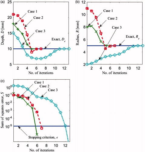
Table 2. Exact tumour parameters D and R and three sets of initial guesses (cases 1, 2 and 3) for the inverse problem with two unknowns (steady state analysis).

	Depth, D (mm)	Radius, R (mm)
Exact	10	5
Case 1
Initial	18	8
Final	10	5
Error (%)	0.002	0.013
Case 2
Initial	21	11
Final	10	5
Error (%)	0.051	0.009
Case 3
Initial	15	2
Final	10	5
Error (%)	0	0.002

Limitations of the steady state analysis

In Section “Steady state analysis with two unknowns (R and D)”, steady state data were used to reconstruct two unknown tumour parameters D and R. In this section, we add a third unknown parameter, the blood perfusion rate ω_b, to the set of unknown tumour parameters, and evaluate the feasibility of simultaneously reconstructing all three parameters from steady state data. The exact values of the tumour parameters for the steady state analysis and the three initial guesses are shown in Table 3. Figure 7 illustrates the progression of the parameters from the initial guess to the final solution. Final solutions along with the corresponding errors are shown in Table 3. For all three cases, the iteratively computed solution progressed away from exact solution. Cases 1 and 2 exhibit large errors, especially for the estimates of ω_b, 83.3% and 40%, respectively. For case 3, the error was smaller, with a maximum error of 7% for ω_b. The smaller error for case 3 can be attributed to the initial guess being very close to the exact solution.

Figure 7. Evolution of (a) depth D (b) radius R (c) blood perfusion rate ω_b of the tumour and the (d) error S(P) versus the number of iterations using steady state data for the three cases in Table 3.

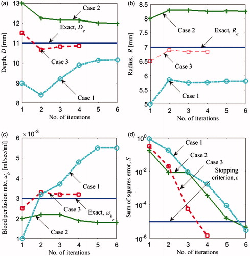
Table 3. Exact parameter values and three sets of initial guesses for the inverse problem with three unknowns for steady state analysis. Temperature rise for sets of parameters marked by * is plotted in Figure 8.

	Depth, D (mm)	Radius, R (mm)	Blood perfusion rate, ωb (m^3/sec/m^3)
Exact*†	11	7	0.003
Case 1
Initial	9	5	0.001
Final*	10.15	5.8	0.0055
Error (%)	7.7	17.1	83.3
Case 2
Initial	13	8	0.002
Final*	12	8.3	0.0018
Error (%)	9.1	18.6	40
Case 3
Initial	11.5	6.5	0.0025
Final	10.9	6.8	0.0032
Error (%)	0.91	2.9	6.67

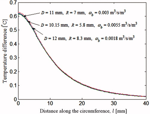
This behaviour of the inverse reconstruction algorithm can be explained by considering the results in Figure 8, which compares the surface temperature profiles of the three tumours. The temperature plotted in Figure 8 is the temperature rise due to the presence of tumour. The temperature difference calculated by subtracting the surface temperature of the healthy breast from the temperature of the cancerous breast. One of the three surface temperature profiles in Figure 8 correspond to the exact set of parameters (†) given in Table 3. The remaining two show the converged, but incorrect, solutions of cases 1 and 2 marked by * in Table 3. In spite of the marked difference in the tumour parameter values D, R and ω_b, the three tumours yield almost identical surface temperature profiles, close enough to satisfy the stopping criterion (Equation (21)(21) . These results suggest that different combinations of D, R and ω_b can yield nearly identical thermal signatures, that is, the thermal signatures of the tumour are not unique. Therefore, during the iterative revisions of the parameter set, the inverse algorithm converged to an incorrect solution. The reduction in surface temperature due to smaller tumour size for the final solution of case 1 is compensated by lower depth and a higher blood perfusion rate of the other tumours.

Figure 8. Surface temperature profiles for tumour parameters marked by * in Table 3.

The analysis in Section “Steady state analysis with two unknowns (R and D)” demonstrates that, based on the steady state analysis, it was possible to estimate the location and the size of the tumour. However, the results in Section “Limitations of the steady state analysis” indicate that it is not possible to estimate the third parameter ω_b. When the blood perfusion rate is included along with size and location as unknown, the inverse problem based on steady state analysis converges to the wrong solutions. Since different tumours yield almost identical surface temperature distributions, the inverse reconstruction algorithm is unable to distinguish between them. This implies that the solution for this inverse problem with three unknowns is not unique, even though the algorithm yields a unique solution for two unknowns. In clinical applications, the presence of noise, can further accentuate the problem.

Solution: transient analysis

To overcome the non-uniqueness problem and solve this inverse problem in a robust manner, we incorporated the transient response in the input data. The transient response has been used in prior studies by Çetingül and Herman [25] for melanoma detection, Cheng and Herman [13] for the analysis of near surface lesions and Bhargava et al. [35] for deep tissue injury. The imaging technique employed in these studies is known as dynamic IR imaging, and it is explained in Section “Mathematical model” (Equation (8)(8) ). In dynamic IR imaging, a cooling load is applied on the surface for a certain amount of time. Then the cooling load is removed and the surface temperature is allowed to recover. The temperature measured during the thermal recovery process is used along with steady state temperature distribution to quantitatively assess lesions.

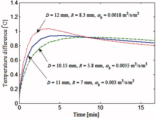
In order to compare surface temperatures generated by different tumours, firstly, the temperature of a cancerous breast is computed during the thermal recovery process, at a point located on the skin surface and on the axis, directly above the tumour. The reason for picking this particular point has been explained in Section “Input data for the inverse problem: computational phantom”. Then the temperature of a healthy breast at the same location is subtracted from it, resulting in a temperature difference. In Figure 9, this temperature difference is plotted against time, for the three tumours considered in the steady state analysis. These are the same three tumours marked by * in Table 3, which resulted in identical steady state surface temperature profiles (Figure 8). It can be seen that the transient thermal recovery temperature profile is different for the three cases. Therefore, the inverse reconstruction algorithm should not get trapped into incorrect solutions when transient data are included in the analysis. This approach makes it possible to estimate the blood perfusion rate along with the size and location of the tumour uniquely.

Figure 9. Thermal recovery temperature profile of a point directly above the tumour corresponding to θ₀. The tumours considered are the 3 tumours marked by * in Table 3 and are also discussed in Figure 7.

Transient analysis with three unknowns

To illustrate the use of transient response in inverse reconstruction we considered the same set of exact parameters E_tr (Equation (10)(10) and initial guesses Y_tr (Equation (13)(13) as for the steady state analysis (Table 3) and added the transient data. A detailed description of the input parameters for the transient case is found in Section “Input data for the inverse problem: computational phantom”. Figure 10 illustrates the progression of the solution from the initial guess to the converged solution for D, R and ω_b. The error for each iteration is shown in Figure 10(d). The solution converged to the correct solution for all three initial guesses, with negligible errors (Table 4). Case 1 took the highest number of iterations to converge (34) and case 3 the least number of iterations (8). Since the blood perfusion rate is an indicator of the metabolic activity of the tumour, it can help estimate the stage of the tumour and therefore it is an important tumour parameter of interest in clinical applications. Furthermore, the use of additional set of input data improves the accuracy of the solution and can reduce the effect of noise in the input data therefore improving the robustness of the solution. In the transient analysis, temperatures were recorded at intervals of more than 100 s and this makes sure that it is easily within the temporal resolution of IR cameras, which is less than a second.

Figure 10. Evolution of (a) depth D (b) radius R (c) blood perfusion rate ω_b of the tumour and (d) error S(P) versus the number of iterations using transient data for the three cases summarised in Table 4.

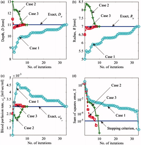
Table 4. Exact parameter values and three sets of initial guesses for the inverse problem with three unknowns for transient analysis.

	Depth, D (mm)	Radius, R (mm)	Blood perfusion rate, ωb (m^3/sec/m^3)
Exact	11	7	0.003
Case 1
Initial	9	5	0.001
Final	11	7	0.003
Error (%)	0.009	0.017	0
Case 2
Initial	13	8	0.002
Final	11	7	0.003
Error (%)	0.004	0.008	0
Case 3
Initial	11.5	6.5	0.0025
Final	11	7	0.003
Error (%)	0.024	0.039	0

Several other cases were tried with different set of exact parameters and are listed in Table 5. Different initial guesses were tried, including those which were far away from the exact parameters. The test cases considered here have tumours ranging from 12 mm to 30 mm in depth, 7 mm to 11 mm in radii and blood perfusion rate ranging from 0.003 1/s to 0.01 1/s. The error in the solution was low for near surface tumours and it increased with increasing depths. It was observed that tumours with 0.01 1/s blood perfusion rate and 11 mm radii gave errors of less than 1% when they are within 20 mm from the body surface. Even though shallower tumours in Table 5 have blood perfusion rates lower than 0.01 1/s and hence lower rise in surface temperature (Figure 5), they were giving low errors. Errors in blood perfusion rate were particularly large for deeper tumours, this can be explained by the fact that surface temperature becomes increasingly insensitive to the blood perfusion rates for deeper tissue layers [28]. Furthermore, smaller tumours will be giving lower temperature signals, but it is the larger tumours which have been associated with lower survival [36].

Table 5. Exact parameter values and sets of initial guesses for the inverse problem with three unknowns for transient analysis.

	Depth, D (mm)	Radius, R (mm)	Blood perfusion rate, ωb (m^3/sec/m^3)
Exact	12	10	0.003
Case 1
Initial	10	8	0.002
Final	12	10	0.003
Error (%)	0.053	0.05	0
Exact	13	10	0.004
Case 1
Initial	12	9	0.003
Final	13	10	0.004
Error (%)	0	0.001	0
Case 2
Initial	10	9	0.003
Final	13	10	0.004
Error (%)	0	0.009	0
Case 3
Initial	12	7	0.003
Final	13	10	0.004
Error (%)	0	0.015	0
Case 4
Initial	10	8	0.005
Final	13	10	0.004
Error (%)	0	0.008	0
Exact	14	10	0.0045
Case 1
Initial	13	11	0.004
Final	14	10	0.0045
Error (%)	0.03	0.068	0
Case 2
Initial	12	9	0.003
Final	14	10	0.0045
Error (%)	0.022	0.082	0
Case 3
Initial	11	8	0.0035
Final	14	10	0.0045
Error (%)	0.02	0.073	0
Case 4
Initial	16	8	0.0025
Final	14	10	0.0045
Error (%)	0.014	0.055	0
Case 5
Initial	10	7	0.002
Final	14	10	0.0045
Error (%)	0.014	0.055	0
Case 6
Initial	8	4	0.001
Final	14	10	0.0045
Error (%)	0.021	0.074	0
Case 7
Initial	21	6	0.003
Final	14	10	0.0045
Error (%)	0.03	0.097	0
Exact	16	11	0.0055
Case 1
Initial	14	9	0.002
Final	16	11	0.0055
Error (%)	0.002	0.014	0
Case 2
Initial	12	7	0.002
Final	16	11	0.0055
Error (%)	0.001	0.006	0
Exact	15	11	0.01
Case 1
Initial	13	9	0.008
Final	15	11	0.010
Error (%)	0.013	0.035	0
Case 2
Initial	12	8	0.007
Final	15	11	0.01
Error (%)	0.001	0.006	0
Case 3
Initial	18	8	0.005
Final	15	11	0.01
Error (%)	0.015	0.042	0
Exact	20	11	0.01
Case 1
Initial	22	9	0.007
Final	20.02	10.90	0.0108
Error (%)	0.1	0.91	8
Exact	25	11	0.01
Case 1
Initial	23	9	0.008
Final	25.07	10.53	0.015
Error (%)	0.28	4.27	50
Case 2
Initial	20	9	0.007
Final	25.10	10.50	0.0157
Error (%)	0.4	4.54	57
Exact	30	11	0.01
Case 1
Initial	28	9	0.008
Final	29.71	10.15	0.0181
Error (%)	0.97	7.73	81
Case 2
Initial	27	8	0.008
Final	29.96	9.8	0.0319
Error (%)	0.13	10.91	219
Case 3
Initial	26	7	0.007
Final	29.59	9.51	0.0332
Error (%)	1.37	13.55	232
Case 4
Initial	20	6	0.005
Final	30.23	9.44	0.0637
Error (%)	0.77	14.18	537

The ability gained by this novel approach to estimate the blood perfusion rate is very critical. MRI, mammography and other non-invasive modalities can identify the location and size of the tumour, but it is difficult to ascertain the level of malignancy of the tumour based on these tumour parameters. The diagnosis of cancer might require multiple visits to the clinic and a biopsy for determination of tumour malignancy. On the other hand, an estimate of blood perfusion rate can give an unequivocal indication of tumour malignancy, as there is a direct correlation between tumour growth rate and tumour malignancy. Therefore, this approach has the potential to reduce the time, cost and effort involved in tumour detection.

Even though this approach, in its present format, does not give accurate result for deeper tumours, it can be modified to give critical diagnostic and staging information. CT scans can be used to determine the location and size of the tumour and this information can then be potentially utilised to increase the accuracy of the blood perfusion rate estimation. Blood perfusion rate in turn can help in staging of the tumour, which is very critical in determining the cancer treatment strategy. It should be noted that MRI can also be used to estimate blood perfusion. MRI can give the blood perfusion distribution within the tissue and it can prove beneficial for diagnosing and characterising tumours. Thermography has an edge over MRI as it is much more economical and completely non-invasive. An MRI system is very expensive and requires a dedicated room or hardware (or large trailers for mobile systems) and a highly trained operator. A thermographic imaging system costs orders of magnitude less, is orders of magnitude smaller and can operated by existing clinical staff after basic training. It is suitable for screening and telemedicine applications. Additionally for MRI perfusion measurements, contrast agent has to be injected into the subject’s body. Thermographic tests can be 10 times cheaper and the equipment cost can be 100 times less than MRI [37].

Noise analysis

The IR cameras available presently have thermal and spatial resolution of 10 mK and 0.05 mm, respectively or better [38]. Although it should be noted that spatial resolution is not a property of the camera and for a certain sensor size, it will depend on the distance of the camera from the object. The points on the body surface, at which the temperatures are measured (Figure 2(c)), are at a distance of 5 mm from each other and the spatial resolution of the IR cameras, at 0.05 mm, is well above this, so they can easily capture the spatio-temperature variation.

For thermal resolution, an analysis has been done here to show the limitations when noise corresponding to 10 mK is present in temperature measurement. A random noise of 10 mK was generated in the temperature data using a MATLAB function. For the noise analysis, the stopping criteria (Equation (21))(21) were relaxed by increasing ɛ to 5 × 10⁻⁴. This particular stopping criteria were chosen based on multiple runs for different cases and selecting an ɛ which will lead to convergence for maximum cases. The results hence generated have been tabulated in Table 6. The set of exact parameters have been taken from Table 5 and corresponding initial guesses are a subset of the cases investigated before in Table 5. It was made sure that the subset of the initial guesses had cases which were farther away from the exact set of parameters and therefore most challenging. As expected the errors associated with the final solution are larger here due to the presence of noise and a relaxed stopping criterion, as compared to the earlier case (Table 5). Here again the error increased with increasing depth of the tumour and the errors in blood perfusion estimates were particularly high for deep tumours.

Table 6. Exact parameter values and sets of initial guesses for the inverse problem with three unknowns for transient analysis. A 10 mK noise was added to the surface temperature and a stopping criterion ɛ = 5 * 10⁻⁴ was used.

	Depth, D (mm)	Radius, R (mm)	Blood perfusion rate, ωb (m^3/sec/m^3)
Exact	11	7	0.003
Case 2
Initial	13	8	0.002
Final	11.09	7.13	0.0029
Error (%)	0.82	1.86	3.33
Case 3
Initial	11.5	6.5	0.0025
Final	11.02	7	0.003
Error (%)	0.18	0	0
Exact	12	10	0.003
Case 1
Initial	10	8	0.002
Final	11.97	9.97	0.003
Error (%)	0.25	0.3	0
Exact	13	10	0.004
Case 2
Initial	10	9	0.003
Final	13.02	10	0.004
Error (%)	0.15	0	0
Case 4
Initial	10	8	0.005
Final	13	9.99	0.004
Error (%)	0	0.1	0
Exact	14	10	0.0045
Case 7
Initial	21	6	0.003
Final	13.89	9.88	0.0046
Error (%)	0.79	1.2	2.22
Exact	16	11	0.0055
Case 1
Initial	14	9	0.002
Final	16.01	8.91	1.82
Error (%)	0.063	8.91	1.82
Exact	15	11	0.01
Case 1
Initial	13	9	0.008
Final	15.01	10.98	0.0102
Error (%)	0.07	0.18	2
Case 2
Initial	12	8	0.007
Final	14.99	10.98	0.0102
Error (%)	0.07	0.18	2
Case 3
Initial	18	8	0.005
Final	15.06	11.06	0.0098
Error (%)	0.4	0.55	2
Exact	20	11	0.01
Case 1
Initial	22	9	0.007
Final	19.57	10.66	0.0101
Error (%)	2.15	3.09	1
Exact	25	11	0.01
Case 1
Initial	23	9	0.008
Final	24.42	10	0.0155
Error (%)	2.32	9.09	55
Case 2
Initial	20	9	0.007
Final	24.57	10.3	0.0132
Error (%)	1.72	6.37	32
Exact	30	11	0.01
Case 1
Initial	28	9	0.008
Final	27.3	9.4	0.0104
Error (%)	9	14.55	4
Case 2
Initial	27	8	0.008
Final	26.33	8.59	0.0116
Error (%)	12.23	21.91	16
Case 3
Initial	26	7	0.007
Final	26.89	8.54	0.0176
Error (%)	10.37	22.36	76
Case 4
Initial	20	6	0.005
Final	27.27	8.35	0.03
Error (%)	9.1	24.09	174

Computational time

The time taken by this algorithm can vary from 10 min to 50 min depending on the number of iterations required for convergence. In general, the further the initial guess is from the actual solution the larger the number of iterations will be as can be seen from Figures 6 and 10. It takes around 75 s for one iteration loop as shown in the flowchart corresponding to the outer loop (Figure 3), if the next set of parameters (Figure 4, block (d)) obtained using Equation (26)(26) is realistic (Figure 4, block (e)) and is a better estimate than the previous one (Figure 4, block (i)). If the estimate is unrealistic (Figure 4, block (e)), it takes a couple of seconds to correct it and if it needs to be improved (Figure 4, block (i)), it takes an extra 20 s for each loop.

Future work

Several improvements can be incorporated into the existing model in the future. First, the LM algorithm can be modified to improve the robustness and speed. Second, a 3D model of the breast can be used to include tumours which are not centred along the axis. Third, the variation in thermophysical properties with temperature can be included in the model to make it more accurate. Finally, a sensitivity analysis can be done to quantify the effect of uncertainties of the parameters involved.

Conclusions

In the present work, we used an inverse reconstruction method, based on the LM algorithm, to characterise a tumour based on the skin surface temperature. This method was applied for two different cases. The first case relied on steady state surface temperature data as input. Tumor location and size were the unknown parameters, and the thermophysical properties of the tumour and healthy tissue were considered to be known. In the second case, transient data served as input along with steady state data, and the blood perfusion rate of the tumour was added to the unknown parameters. A multilayered 2 D model of the breast was considered for the present analysis.

The first case, that uses the surface temperature profile at steady state, has some limitations. Though it can uniquely estimate size and location of the tumour based on steady state data, problem arises when an additional tumour parameter, blood perfusion rate, is added as an unknown. Noise in the input data can further accentuate the problem. In order to correctly and uniquely estimate the size, location and blood perfusion rate of the tumour simultaneously, we used transient analysis in the second case. For deeper tumours, the solution seems to converge away from the exact set of parameters.

To summarise, addition of transient data with steady state data allows simultaneous estimation of blood perfusion rate, size and location of tumour, which is not possible with steady state data alone. Although this has limitations, but when combined with other modalities it can help in staging and treatment planning for cancer.

Acknowledgements

We gratefully acknowledge the support for Rajeev Hatwar by the Department of Mechanical Engineering, Johns Hopkins University.

Disclosure statement

The authors report no conflicts of interest. The authors alone are responsible for the content and writing of the article.

Additional information

Funding

Partial support for Rajeev Hatwar and Cila Herman was provided by the National Institutes of Health, NCI Grant No. R01CA161265.

References

- Lee CH, Dershaw DD, Kopans D, et al. (2010). Breast cancer screening with imaging: recommendations from the Society of Breast Imaging and the ACR on the use of mammography, breast MRI, breast ultrasound, and other technologies for the detection of clinically occult breast cancer. JACR 7:18–27.
- Kennedy DA, Lee T, Seely D. (2009). A comparative review of thermography as a breast cancer screening technique. Integr Cancer Ther 8:9–16.
- Ng EYK. (2009). A review of thermography as promising non-invasive detection modality for breast tumor. Int J Therm Sci 48:849–59.
- Lawson R. (1956). Implications of surface temperatures in the diagnosis of breast cancer. CMAJ 75:309–11.
- Gautherie M, Gros CM. (1980). Breast thermography and cancer risk prediction. Cancer 45:51–6.
- Gautherie M. (1980). Thermopathology of breast cancer: measurement and analysis of in vivo temperature and blood flow. Ann NY Acad Sci 335:383–415.
- Weidner N, Folkman J, Pozza F, et al. (1992). Tumor angiogenesis: a new significant and independent prognostic indicator in early-stage breast carcinoma. Cancer Spectr Know Environ 84:1875–87.
- Zetter BR. (1998). Angiogenesis and tumor metastasis. Annu Rev Med 49:407–24.
- Yahara T, Koga T, Yoshida S, et al. (2003). Relationship between microvessel density and thermographic hot areas in breast cancer. Surg Today 33:243–8.
- Krüger K, Stefansson IM, Collett K, et al. (2013). Microvessel proliferation by co-expression of endothelial nestin and Ki-67 is associated with a basal-like phenotype and aggressive features in breast cancer. Breast 22:282–8.
- Çetingül MP, Herman C. (2010). A heat transfer model of skin tissue for the detection of lesions: Sensitivity analysis. Phys Med Biol 55:5933–51.
- Chanmugam A, Hatwar R, Herman C. (2012). Thermal analysis of cancerous breast model. Proc. ASME 2012 Int. Mech. Engg. Congress and Exposition Conf., Houston, Texas, USA; 2012 Nov 9: 135–143.
- Cheng TY, Herman C. (2014). Analysis of skin cooling for quantitative dynamic infrared imaging of near-surface lesions. Int J Therm Sci 86:175–88.
- Mital M, Pidaparti RM. (2008). Breast tumor simulation and parameters estimation using evolutionary algorithms. Model Simul Eng 2008:756436.
- Mitra S, Balaji C. (2010). A neural network based estimation of tumour parameters from a breast thermogram. Int J Heat Mass Tran 53:4714–27.
- Bezerra LA, Oliveira MM, Rolim TL, et al. (2013). Estimation of breast tumor thermal properties using infrared images. Signal Process 93:2851–63.
- Tepper M, Shoval A, Hoffer O, et al. (2013). Thermographic investigation of tumor size, and its correlation to tumor relative temperature, in mice with transplantable solid breast carcinoma. J Biomed Opt 18:111410.
- Das K, Mishra SC. (2013). Estimation of tumor characteristics in a breast tissue with known skin surface temperature. J Therm Biol 38:311–317.
- Das K, Mishra SC. (2014). Non-invasive estimation of size and location of a tumor in a human breast using a curve fitting technique. Int Commun Heat Mass Transfer 56:63–70.
- Das K, Mishra SC. (2015). Simultaneous estimation of size, radial and angular locations of a malignant tumor in a 3-D human breast – a numerical study. J Therm Biol 52:147–156.
- Rodrigues HF, Mello FM, Branquinho LC, et al. (2013). Real-time infrared thermography detection of magnetic nanoparticle hyperthermia in a murine model under a non-uniform field configuration. Int J Hyperthermia 29:752–767.
- Dabbagh A, Abdullah BJ, Abu Kasim NH, Ramasindarum C. (2014). Reusable heat-sensitive phantom for precise estimation of thermal profile in hyperthermia application. Int J Hyperthermia 30:66–74.
- Pennes HH. (1948). Analysis of tissue and arterial blood temperatures in the resting human forearm. J Appl Physiol 1:93–122.
- Ozisik MN, Orlande H. (2000). Inverse heat transfer: fundamentals and applications. New York: Taylor and Francis, 3–112.
- Çetingül MP, Herman C. (2011). Quantification of the thermal signature of a melanoma lesion. Int J Therm Sci 50:421–431.
- Deng ZS, Liu J. (2000). Parametric studies on the phase shift method to measure the blood perfusion of biological bodies. Med Eng Phys 22:693–702.
- Liu J, Zhou YX, Deng ZS. (2002). Sinusoidal heating method to noninvasively measure tissue perfusion. IEEE Trans Biomed Eng 49:867–877.
- Kleinman AM, Roemer RB. (1983). A direct substitution, equation error technique for solving the thermographic tomography problem. J Biomech Eng 105:237–243.
- Bhowmik A, Repaka R. (2016). Estimation of growth features and thermophysical properties of melanoma within 3-D human skin using genetic algorithm and simulated annealing. Int J Heat Mass Tran 98:81–95.
- Comsol Multiphysics (2013). Version 4.3 Comsol Inc. Available from: https://www.comsol.com/comsol-multiphysics
- Ng EY, Sudharsan NM. (2001). An improved three-dimensional direct numerical modelling and thermal analysis of a female breast with tumour. Proc Inst Mech Eng H J Eng Med 215:25–37.
- Amri A, Saidane A, Pulko S. (2011). Thermal analysis of a three-dimensional breast model with embedded tumour using the transmission line matrix (TLM) method. Comput Biol Med 41:76–86.
- Jiang L, Zhan W, Loew MH. (2010). Modeling static and dynamic thermography of the human breast under elastic deformation. Phys Med Biol 56:187–202.
- Cheng TY. (2015). Improving quantitative infrared imaging for medical diagnostic applications [Doctoral dissertation]. Baltimore (MD): Johns Hopkins University.
- Bhargava A, Chanmugam A, Herman C. (2014). Heat transfer model for deep tissue injury: a step towards an early thermographic diagnostic capability. Diagn Pathol 9:36.
- Carter CL, Allen C, Henson DE. (1989). Relation of tumor size, lymph node status, and survival in 24,740 breast cancer cases. Cancer 63:181–187.
- Arora N, Martins D, Ruggerio D, et al. (2008). Effectiveness of a noninvasive digital infrared thermal imaging system in the detection of breast cancer. Am J Surg 196:523–526.
- Çetingül MP. (2010). Using high resolution infrared imaging to detect melanoma and dysplastic nevi [Doctoral dissertation]. Baltimore (MD): Johns Hopkins University.