Estimation of the temperature field in laser-induced hyperthermia experiments with a phantom

Abstract

Background: One of the challenges faced during the hyperthermia treatment of cancer is to monitor the temperature distribution in the region of interest. The main objective of this work was to accurately estimate the transient temperature distribution in the heated region, by using a stochastic heat transfer model and temperature measurements.

Methods: Experiments involved the laser heating of a cylindrical phantom, partially loaded with iron oxide nanoparticles. The nanoparticles were manufactured and characterized in this work. The solution of the state estimation problem was obtained with an algorithm of the Particle Filter method, which allowed for simultaneous estimation of state variables and model parameters. Measurements of one single sensor were used for the estimation procedure, which is highly desirable for practical applications in order to avoid patient discomfort.

Results: Despite the large uncertainties assumed for the model parameters and for the coupled radiation–conduction model, discrepancies between estimated temperatures and internal measurements were smaller than 0.7 °C. In addition, the estimated fluence rate distribution was physically meaningful. Maximum discrepancies between the prior means and the estimated means were of 2% for thermal conductivity and heat transfer coefficient, 4% for the volumetric heat capacity and 3% for the irradiance.

Conclusions: This article demonstrated that the Particle Filter method can be used to accurately predict the temperatures in regions where measurements are not available. The present technique has potential applications in hyperthermia treatments as an observer for active control strategies, as well as to plan personalized heating protocols.

Keywords:

• State estimation
• particle filter
• Monte Carlo
• nanoparticles

Introduction

The use of heat for therapeutic purposes in medicine dates back from remote centuries [1–3]. The hyperthermia treatment of cancer requires heat deposition in tumorous tissues with minimum heating of healthy cells. With the recent developments in nanotechnology, nanoparticles have been concentrated in the tumor to locally increase the absorption of electromagnetic waves imposed by energy sources [4]. In the case of near-infra-red laser-induced hyperthermia, noble metal nanoparticles, nanopolymers and oxide nanoparticles, with high optical absorption, were used as thermal agents in several reported studies [5–7].

One of the challenges faced during the hyperthermia treatment of cancer is to monitor the temperature distribution in the region of interest. Temperature measurement techniques available nowadays can be classified as invasive and noninvasive [8,9]. Noninvasive techniques are generally contact free, do not require the sensors to be inserted into the body and can provide a three-dimensional map of the temperature field. Currently, magnetic resonance temperature imaging (MRTI) via proton resonance frequency shift is the most advanced non-invasive temperature measurement technique, but its widespread use in clinics is still limited [8–11]. In contrast, the sensors are inserted into the body in invasive techniques. Thus, the number of sensors must be kept small for minimising patient discomfort. Fiber optic sensors were used for internal temperature measurements during breast hyperthermia treatment by Notter et al. [12], while Schena et al. [9] provided an overview on the types of fiber optic sensors used for invasively monitoring hyperthermia.

Regardless of the measurement technique, whether invasive or noninvasive, the measured temperatures do contain uncertainties. Likewise, tissue properties exhibit a large variability that must be accounted for in numerical simulations required for the planning and the predictive control of the hyperthermia treatment [13–20]. Bayesian state estimation techniques provide a systematic framework for combining uncertainties in the measured data and in the mathematical model of the physical problem [15–18]. Such techniques result in accurate estimates of the temperature distribution inside the body, thermal dose and thermal damage [21] during the hyperthermia treatment of cancer [13,15–18]. In the case of invasive temperature monitoring, where the number of measurement points must be small, such a methodology can be useful for providing an estimate of the transient spatial distribution of the temperature in the region of interest.

Bayesian state estimation formulation of the hyperthermia treatment of cancer was shown to provide accurate estimates of state variables, for cases involving synthetic measured data [13,15–18]. In these works, Particle Filter Methods [22–29], also referred to as Sequential Monte Carlo Methods, were used for the solution of state estimation problems related to the hyperthermia treatment of cancer, with heating in the near-infra-red or radiofrequency ranges. Here, we focus on the experimental validation of the state estimation approach advanced by our group [13,15–18], for the case of the near-infra-red heating of a cylindrical phantom. A tumor was simulated inside the phantom by a disk that contained iron oxide nanoparticles, which were used to promote a localized absorption of the near-infra-red laser beam. The state estimation problem was solved using transient temperature measurements available at a single position within the phantom and a coupled radiation—heat conduction evolution model. The transient temperature distribution within the phantom was estimated together with the laser fluence rate distribution, as well as with the parameters that appear in the mathematical formulation of the problem.

Materials and methods

Experiment

The experiment consisted of a cylindrical plastic phantom that contained a disk-shaped region loaded with nanoparticles. Such a region was aimed at promoting localized heating under near-infra-red laser exposure. The material used for the preparation of the phantom was PVCP (Polyvinyl Chloride Plastisol, M-F Manufacturing Co., Fort Worth, TX). Iron oxide nanoparticles were used as the laser absorbing agent due to their relative low cost.

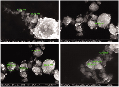
The nanoparticles were manufactured by loading iron oxide (Fe₂O₃ powder with particles smaller than 5 μm, bought from Sigma-Aldrich, Co) into a planetary ball mill (Fritsch GmbH Pulvirisette 6), where hardened steel vials with 257.65 cm³ containing six stainless steel balls of 22 mm diameter, were set in rotation at 600 rpm. The ball-to-powder mass ratio was 30:1 [30]. Milling was performed in a dry air atmosphere for 24 h. X-ray diffraction measurements of the produced nanoparticles were performed in an XRD Bruker D8 Discover, with Co (Kα) radiation in the 2θ range from 20° to 90°. The morphology and size of the nanoparticles were observed by Field emission gun-scanning electron microscopy in a FEG-MEV model FEI Versa 3D. Typical X-ray powder diffraction patterns of the iron oxide particles, before and after milling, are shown by Figure 1. The diffraction patterns are consistent with Fe₂O₃, thus indicating that the milling process did not affect the chemical structure of the initial sample. Furthermore, the XRD diffractogram has relative sharp peaks, indicating an excellent crystallinity of the samples. For the milled samples, the peaks are broad and with small intensity, indicating the presence of nanoparticles [31]. Figure 2 presents SEM micrographs of the nanoparticles, where it can be noticed agglomerates varying from 30 to 100 nm in size.

Figure 1. X-ray powder diffraction patterns.

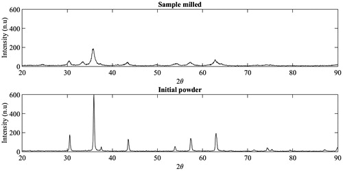
Figure 2. FEG-SEM micrographs of the milled sample.

For the preparation of the phantom, 30 mg of the manufactured Fe₂O₃ nanoparticles were mixed with 25 ml of pure PVCP (concentration of 24% vol) and stirred with an ultrasonic mixer (Cole Parmer, 750 W) for 15 min. Afterwards, the mixture was heated in an oven at 170 °C for one hour and then allowed to naturally cool down at room temperature in a disk-shaped mould, with diameter of 28 mm and thickness of 6 mm. The top and bottom of the mould containing the mixture were covered with glass plates to obtain flat surfaces. The PVCP disk loaded with Fe₂O₃ nanoparticles was then placed in another larger cylindrical mould, with diameter of 40 mm and height of 44 mm. Finally, pure liquid PVCP at 170 °C was poured into the cylindrical mould containing the disk loaded with nanoparticles, to fill the void spaces. Figure 3(a) shows a top view of the phantom, where the disk loaded with nanoparticles appears in brown at the centre. Thermocouple wires can also be seen in this figure.

Figure 3. (a) Top view of the phantom with thermocouples; (b) Experimental setup; (c) Snapshot of the infra-red camera readings.

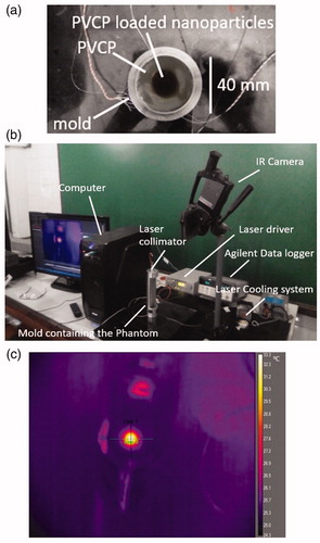
A near-infra-red laser diode (Oclaro) with a mean wavelength of 829.1 nm was used to heat the phantom. The laser diode was connected to a collimator F-H10-NIR-FC (Newport) by an optical fiber. The laser output power was controlled by a laser driver (model 525B, Newport) with a maximum output power of 600 mW. The laser diode was cooled to avoid excessive heating. Light reflection from the bottom of the phantom was minimized by using a support with very low reflectivity. The collimator was coaxially located 15 cm above the phantom. In the experiments, the laser diode was set to deliver two output powers (P₁ = 156.6 mW and P₂ = 220 mW) on continuous wave mode through the collimator. A digital power meter and an infra-red card (Thorlabs) were used for the measurement of the laser output power and spot size, respectively. The phantom was exposed to the laser for 100 s in all experiments. During irradiation, an infra-red thermographic camera (FLIR Thermacam SC660), placed at 80 cm above the phantom, was used to measure its top surface temperature. Also, three thermocouples type K, located at the phantom axis at different depths below the irradiated surface, were used to measure local temperature variations. The thermocouples were placed below the region loaded with nanoparticles (where the absorption coefficient is high) in order to avoid direct laser heating. One of the thermocouples was placed at the back surface of the disk with Fe₂O₃ nanoparticles, at a depth of 8 mm below the top surface of the phantom. The other thermocouples were located at 10 and 15 mm below the top surface of the phantom. The thermocouples were connected to a data acquisition system (AGILENT 34970A) controlled by a computer, which provided readings with a frequency of 1 Hz. The experimental setup and a snapshot of the infra-red camera measurements are shown by Figures 3(b) and 3(c), respectively.

The transient temperature measurements from a single thermocouple and a computational model describing the physics of the problem were jointly used in an inverse analysis. The objective was to provide sequential estimates of the temperature distribution inside the phantom, as described below.

Physical problem and mathematical formulation

The physical problem corresponding to the experiment involves the heating of a cylindrical medium by an external collimated Gaussian laser beam. The laser beam is coaxial with the phantom, so that the problem can be formulated as two-dimensional and axisymmetric. The cylinder made of PVCP contains a coaxial disk inclusion, which simulates the tumor and is made of PVCP loaded with Fe₂O₃ nanoparticles, as illustrated by Figure 4. The dimensions of the phantom and the locations of the thermocouples are also shown in this figure.

Figure 4. Sketch of the phantom with its associated dimensions, laser beam, thermocouples and IR camera.

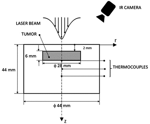
By assuming that absorption dominates scattering in the phantom, the laser light propagation was modeled with Beer–Lambert’s law. The light propagation model was then coupled to a transient heat conduction problem. The surface exposed to the laser radiation (at z = 0) exchanged heat with the surrounding media at T = T₀ by convection and linearized radiation, while the surface at z = L_z was maintained at a prescribed constant temperature T = T₀. Heat transfer was neglected through the lateral surfaces of the phantom. The medium was assumed at a constant uniform initial temperature, T₀. The validity of the hypotheses made for the mathematical formulation is addressed in the discussions of this work.

The heat conduction problem in terms of temperature increase,

T*(r,z,t) = T(r,z,t) – T₀, is then formulated by using position-dependent properties as: (1.a) $$C\left(r,z\right)\frac{\partial T^{*}\left(r,z,t\right)}{\partial t}=\nabla \cdot \left[k\left(r,z\right)\nabla T^{*}\left(r,z,t\right)\right]+Q_{\mathit{\text{laser}}}\left(r,z\right),\hspace{0.17em}\hspace{0.17em}0<z<L_z,0\le r<L_r,\hspace{0.17em}t>0$$(1.a) (1.b) $$-k\frac{\partial T^{*}}{\partial z}+h{T}^{*}=0,\hspace{0.17em}\hspace{0.17em}z=0,\hspace{0.17em}\hspace{0.17em}0\le r\hspace{0.17em}<\hspace{0.17em}{L}_r,\hspace{0.17em}t\hspace{0.17em}>\hspace{0.17em}0$$(1.b) (1.c) $$T^{*}=0,\hspace{0.17em}\hspace{0.17em}z=L_z,\hspace{0.17em}\hspace{0.17em}0\le r\hspace{0.17em}<\hspace{0.17em}{L}_r,\hspace{0.17em}t\hspace{0.17em}>\hspace{0.17em}0$$(1.c) (1.d) $$\frac{\partial T^{*}}{\partial r}=0,\hspace{0.17em}\hspace{0.17em}r=L_r,\hspace{0.17em}\hspace{0.17em}0\hspace{0.17em}<\hspace{0.17em}z\hspace{0.17em}<\hspace{0.17em}\hspace{0.17em}{L}_z,\hspace{0.17em}t\hspace{0.17em}>\hspace{0.17em}0$$(1.d) (1.e) $$T^{*}=0,\hspace{1em}0\hspace{0.17em}<\hspace{0.17em}z\hspace{0.17em}<\hspace{0.17em}{L}_z,\hspace{0.17em}\hspace{0.17em}0\le r\hspace{0.17em}<\hspace{0.17em}{L}_r,\hspace{0.17em}\hspace{0.17em}t=0$$(1.e) where C is the volumetric heat capacity, k is the thermal conductivity and h is the combined heat transfer coefficient for convection and linearised radiation at the surface z = 0. In Equation (1a)(1.a) $$C\left(r,z\right)\frac{\partial T^{*}\left(r,z,t\right)}{\partial t}=\nabla \cdot \left[k\left(r,z\right)\nabla T^{*}\left(r,z,t\right)\right]+Q_{\mathit{\text{laser}}}\left(r,z\right),\hspace{0.17em}\hspace{0.17em}0<z<L_z,0\le r<L_r,\hspace{0.17em}t>0$$(1.a) , the volumetric heat source term Q_laser is due to the laser absorption within the phantom and is given by: (2) $$Q_{\mathit{\text{laser}}}\left(r,z\right)=\kappa \left(r,z\right)\Phi \left(r,z\right)$$(2) where $\kappa$ is the local absorption coefficient and the fluence rate, $\Phi (r,z)$, follows Beer-Lambert's law, that is, (3.a) $$\Phi \left(r,z\right)={\Phi }_i\left(r,z\right)={\Phi }_{0,i-1}\left(r,d_{i-1}\left(r\right)\right)\hspace{0.17em}\text{exp}\hspace{0.17em}\left[-{\kappa }_i\left(z-z_i\right)\right]$$(3.a)

The subscript i refers to the material layer i, d_i is the thickness of each layer, while $z_i$ and ${\Phi }_{0,i-1}$ are the axial position at which the collimated light enters layer i and the collimated fluence rate at this position, respectively. For i = 1 we have: (3.b) $${\Phi }_1\left(r,z\right)=E_0\hspace{0.17em}\text{exp}\hspace{0.17em}\left(-2r^2/r_0^2\right)\hspace{0.17em}\text{exp}\hspace{0.17em}\left(-{\kappa }_{1}z\right)$$(3.b) where r₀ is the Gaussian beam radius, that is, the radial location where the irradiance falls to 1/e² of the maximum irradiance and is related to the Full Width Half Maximum (FWHM) by (3.c) $$r_0=\frac{\mathit{\text{FWHM}}}{\sqrt{2\hspace{0.17em}\text{ln}\hspace{0.17em}2}}$$(3.c)

State estimation problem

Two kinds of problems can be associated to the mathematical formulation given by Equations (1) to (3): a direct problem and an inverse problem. In the direct problem, all the optical and thermophysical properties, boundary conditions, initial condition and the heat source term are known. The objective of the direct problem is to obtain the fluence rate and the transient temperature distribution within the medium. On the other hand, in this work we define an inverse problem of temperature field estimation, given transient temperature measurements taken at single location within the medium. The kind of inverse problem addressed here falls into the class of state estimation problems, which are quite common in science and engineering [22–29].

In a state estimation problem, the mathematical modeling of the physical phenomena and available measurements are combined, in order to sequentially estimate the state variables of interest [22–29,32–34]. State estimation problems are formulated within the Bayesian framework, in order to cope with the different sources of uncertainties present in the mathematical formulation of the physical problem and in the measurements [22–29,32–34].

The definition of the state estimation problem requires two models: a state evolution model, which describes the dynamics of the state variables, and an observation model, which relates the state variables to the available measurements [22–29,32–34]. Let x_k denote the state vector, which contains all the variables that uniquely describe the system at a given time instant t_k. The state evolution model and the observation model can be respectively written in terms of the general vector functions f_k and g_k as [22–29,32–34]: (4.a) $${\mathbf{x}}_k={\mathbf{f}}_k\left({\mathbf{x}}_{k-1},\mathbf{\theta },{\mathbf{v}}_{k-1}\right),\hspace{0.17em}\hspace{0.17em}k=1,\dots ,M$$(4.a) (4.b) $${\mathbf{z}}_k={\mathbf{g}}_k\left({\mathbf{x}}_k,\mathbf{\theta },{\mathbf{n}}_k\right),\hspace{0.17em}\hspace{0.17em}k=1,\dots ,M$$(4.b)

The vector $\mathbf{\theta }$ contains all the non-dynamic parameters of the models, while v_k and n_k represent the noises in the state evolution model and in the observation model, respectively.

The goal of the state estimation problem is to sequentially estimate the posterior probability density $\pi ({\mathbf{x}}_k|{\mathbf{z}}_{1:k},\mathbf{\theta })$ of the state variables, or the joint posterior probability density $\pi ({\mathbf{x}}_k,\mathbf{\theta }|{\mathbf{z}}_{1:k})$ of the non-dynamic parameters and of the state variables, given the measurements ${\mathbf{z}}_{1:k}=\left[{\mathbf{z}}_1,{\mathbf{z}}_2,\dots ,{\mathbf{z}}_k\right]$. Inference on the joint posterior density $\pi ({\mathbf{x}}_k,\mathbf{\theta }|{\mathbf{z}}_{1:k})$ is of practical interest, since the non-dynamic parameters appearing in the models might be unknown or known under uncertainties. Given the state evolution and observation models, as well as the initial distributions of parameters and state variables, the solution of the joint parameter and state estimation problem can be obtained with Bayesian filters. In this work, the Particle Filter algorithm of Liu and West was applied because of its robustness and because it allows that model parameters be simultaneously estimated with state variables [17,18,28,29,35,36].

The Particle Filter method is a Monte Carlo technique for the solution of state estimation problems, in which the posterior probability density function is represented by a set of random samples (particles) with associated weights. As the number of Monte Carlo samples becomes large, it is expected that they provide an appropriate representation of the posterior probability density function and the solution approaches the optimal Bayesian estimate. The Particle Filter algorithms generally make use of an importance density, which is a probability density function proposed to represent another one that cannot be exactly computed, that is, the sought posterior density in the present case. Then, samples are drawn from the importance density instead of the actual density [22–29,32–34].

For the simultaneous estimation of state variables and non-dynamic parameters, let $\{{\mathbf{x}}_k^i,{\mathbf{\theta }}_k^i\}$ denote the particle i at time t_k, with associated weight $w_k^i,i=1,\dots ,N$, where N is the number of particles. The subscript k for the parameter vector $\mathbf{\theta }$ does not represent a time dependence of such quantity, but the fact that it is also estimated sequentially, like the state variables x. The weights are normalized so that ${\sum }_{i=1}^N{w}_k^i=1$. The posterior probability distribution of the state variables and of the parameters at t_k can be discretely approximated by [37–39]: (5) $$\pi \left({\mathbf{x}}_k,{\mathbf{\theta }}_k|{\mathbf{z}}_{1:k}\right)\approx \sum _{i=1}^N{w}_k^i\delta \left({\mathbf{x}}_k-{\mathbf{x}}_k^i\right)\delta \left({\mathbf{\theta }}_k-{\mathbf{\theta }}_k^i\right)$$(5)

Where $\delta (.)$ is the Dirac delta function.

The algorithm of Liu and West for the Particle Filter is based on West's hypothesis [40] of a Gaussian mixture for the vector of parameters θ [28,29,40], that is, (6) $$\pi (\mathbf{\theta }|{\mathbf{z}}_{1:k-1})\hspace{0.17em}\approx \hspace{0.17em}\sum _{i=1}^N{w}_{k-1}^{i}N(\mathbf{\theta }|{\mathbf{m}}_{k-1}^i,h^2{\mathbf{V}}_{k-1})$$(6) where $N(\cdot |\mathbf{m},\mathbf{S})$ is a Gaussian density with mean m and covariance matrix S, while h is a smoothing parameter. Equation (6)(6) $$\pi (\mathbf{\theta }|{\mathbf{z}}_{1:k-1})\hspace{0.17em}\approx \hspace{0.17em}\sum _{i=1}^N{w}_{k-1}^{i}N(\mathbf{\theta }|{\mathbf{m}}_{k-1}^i,h^2{\mathbf{V}}_{k-1})$$(6) shows that the density $\pi (\mathbf{\theta }|{\mathbf{z}}_{1:k-1})$ is a mixture of Gaussian distributions weighted by the sample weights $w_{k-1}^i$. The kernel locations are specified by using the following shrinkage rule [28,37]: (7) $${\mathbf{m}}_{k-1}^i=A\hspace{0.17em}\hspace{0.17em} {\mathbf{\theta }}_{k-1}^i+(1-A) {\overline{\mathbf{\theta }}}_{k-1}$$(7) where $A=\sqrt{1-h^2}$ and ${\overline{\mathbf{\theta }}}_{k-1}$ is the mean of θ at time t_k-1. The shrinkage factor, A, is computed as [28,37]: (8) $$A=\frac{3 \epsilon -1}{2 \epsilon }$$(8) where 0.95 <ε < 0.99.

The steps of Liu and West's particle filter algorithm [28,37], as applied for the advancement of the particles from time t_k-1 to time t_k, are presented in Table 1.

Table 1. Liu and West’s algorithm [28].

Step 1

Find the mean ${\overline{\mathbf{\theta }}}_{k-1}$ of the parameters $\mathbf{\theta }$ at time tk–1.

Step 2

For i = 1,…,N compute ${\mathbf{m}}_{k-1}^i$ with Equation (7)(7) $${\mathbf{m}}_{k-1}^i=A\hspace{0.17em}\hspace{0.17em} {\mathbf{\theta }}_{k-1}^i+(1-A) {\overline{\mathbf{\theta }}}_{k-1}$$(7) , draw new particles ${\mathbf{x}}_k^i$ from the prior density π(xk|${\mathbf{x}}_{{{}_k}_{-1}}^i$,${\mathrm{m}}_{k-1}^i$) and then calculate the mean ${\mu }_k^i$ of xk. Use the likelihood density to calculate the corresponding weights w^ik = π(zk|${\mathbf{\mu }}_k^i$,${\mathbf{m}}_{k-1}^i$)w^ik–1.

Step 3

Calculate the total weight t = Σi w^ik and then normalise the particle weights, that is, for i = 1,…, N let w^ik = t^–1 w^ik .

Step 4

Resample the particles as follows:

Construct the cumulative sum of weights (CSW) by computing ci = ci–1 + w^ik for i = 1,…, N, with c0 = 0

Let i = 1 and draw a starting point u1 from the uniform distribution U[0,N^-1]

For j = 1,…,N

Move along the CSW by making uj = u1 + N^−1(j−1)

While uj > ci make i = i + 1

Assign samples ${\mathbf{x}}_{{{}_k}_{-1}}^j={\mathbf{x}}_{{{}_k}_{-1}}^i$, ${\mathbf{m}}_{{{}_k}_{-1}}^j={\mathbf{m}}_{{{}_k}_{-1}}^i$and ${\mathbf{\mu }}_{{}_k}^j={\mathbf{\mu }}_{{}_k}^i$

Assign parent ij = i

Step 5

For j = 1,…, N draw samples ${\mathbf{\theta }}_k^j$ from $N({\mathbf{\theta }}_k^j|{\mathbf{m}}_{k-1}^{ij},h^2{\mathbf{V}}_{k-1})$, by using the parent ij

Step 6

For j = 1,…, N draw particles ${\mathbf{x}}_{{}_k}^j$ from the prior density π(xk|${\mathbf{x}}_{{}_{k-1}}^{ij}$,${\mathbf{\theta }}_k^j$), by using the parent ij, and then use the likelihood density to calculate the correspondent weights $w_k^j$ = π(zk|${\mathbf{x}}_k^j$,${\mathbf{\theta }}_k^j$)/π(zk|${\mathbf{\mu }}_{{}_k}^{ij}$,${\mathbf{m}}_{{}_{k-1}}^{ij}$)

Step 7

Calculate the total weight t = Σj$w_k^j$ and then normalise the particle weights, that is, for j = 1,…, N let $w_k^j$ = t^–1 $w_k^j$

In this work, the vector of state variables at time t_k, ${\mathbf{x}}_k$, includes the fluence rates and temperatures at the centers of the discretized finite volumes, which were used for the solution of the forward problem, represented by the vectors ${\mathbf{\Phi }}_k$ and ${\mathbf{T}}_k$, respectively. The state estimation problem aims at obtaining the spatial distribution of the fluence rate and transient temperature distribution in the phantom, given transient temperature measurements available from one single thermocouple. For the results presented in this article, only the transient measurements obtained with the thermocouple located at the position (r = 0, z = 8) mm were used for the solution of the state estimation problem. Since the physical properties and the laser flux are known with a certain degree of uncertainty, they are jointly estimated with the fluence rate and temperature fields.

For solving this problem with Liu and West’s Particle Filter algorithm, we assume Gaussian additive uncertainties for the state evolution model and for the observation model. The state evolution model is given by: (9) $${\mathbf{x}}_k={\mathbf{f}}_k\left({\mathbf{x}}_{k-1},{\mathbf{\theta }}_{k-1},{\mathbf{v}}_{k-1}\right)=\left[\begin{array}{c}{\mathbf{\Phi }}_k\\ {\mathbf{T}}_k\end{array}\right]=\left[\begin{array}{l}{\mathbf{f}}_k^{rad}\left({\mathbf{\theta }}_{k-1}^{rad}\right)+{\sigma }_{\Phi }{\mathbf{\epsilon }}_k^{\Phi }\\ {\mathbf{f}}_k^{\mathit{\text{cond}}}\left({\mathbf{T}}_{k-1},{\mathbf{\Phi }}_k,{\mathbf{\theta }}_{k-1}^{\mathit{\text{cond}}}\right)+{\sigma }_T{\mathbf{\epsilon }}_k^T\end{array}\right]$$(9)

In Equation (9)(9) $${\mathbf{x}}_k={\mathbf{f}}_k\left({\mathbf{x}}_{k-1},{\mathbf{\theta }}_{k-1},{\mathbf{v}}_{k-1}\right)=\left[\begin{array}{c}{\mathbf{\Phi }}_k\\ {\mathbf{T}}_k\end{array}\right]=\left[\begin{array}{l}{\mathbf{f}}_k^{rad}\left({\mathbf{\theta }}_{k-1}^{rad}\right)+{\sigma }_{\Phi }{\mathbf{\epsilon }}_k^{\Phi }\\ {\mathbf{f}}_k^{\mathit{\text{cond}}}\left({\mathbf{T}}_{k-1},{\mathbf{\Phi }}_k,{\mathbf{\theta }}_{k-1}^{\mathit{\text{cond}}}\right)+{\sigma }_T{\mathbf{\epsilon }}_k^T\end{array}\right]$$(9) , the evolution models for the temperature and fluence rate were represented separately, where ${\mathbf{f}}_k^{rad}$ and ${\mathbf{f}}_k^{\mathit{\text{cond}}}$ are given by the discrete forms of Equations (3) and (1), respectively. The vectors ε^Φ and ε^Τ are uncorrelated Gaussian variables, with zero mean and unitary standard deviations, while the standard deviations for the temperature and fluence rate models are given by ${\sigma }_T=$ 0.5 °C and ${\sigma }_{\Phi }$ = 1% of the fluence’s deterministic value, respectively. The vectors of parameters ${\mathbf{\theta }}_{}^{rad}$ and ${\mathbf{\theta }}_{}^{\mathit{\text{cond}}}$ contain the optical and thermophysical properties, respectively. The initial distributions of the state variables at time t = 0 were also assumed Gaussian, with zero means and the standard deviations given above. For the results presented below, 2000 particles were used in the computations with the Particle Filter.

The prior probability densities for the model parameters at time t = 0 were assumed Gaussian, centered on values obtained from independent measurements made in this work, or taken from the literature. The C-Therm TCi Thermal Conductivity Analyzer (C-Therm Tecnologies), which is based on the modified transient plane source technique, was used to measure the thermal conductivity and the thermal effusivity of both pure PVCP and of the PVCP disk containing the iron oxide nanoparticles. The measured thermal conductivity values were (0.21 $\pm$ 0.01) W m⁻¹ K⁻¹ and (0.22 $\pm$ 0.01) W m⁻¹ K⁻¹, for pure PVCP and for PVCP containing Fe₂O₃ nanoparticles, respectively. The volumetric heat capacities were directly calculated from the measured thermal conductivities and thermal effusivities as (1.4989 $\pm$ 0.0003) MJ m⁻³ K⁻¹ and (1.4755 $\pm$ 0.0003) MJ m⁻³ K⁻¹, for pure PVCP and for PVCP with nanoparticles, respectively. The mean value for the absorption coefficient of the pure PVCP was taken from the literature [41,42]. For the absorption coefficient of the PVCP disk containing nanoparticles, the prior mean value was assigned by comparing the surface temperatures measured on the surface of the heated phantom with numerical simulations of the forward problem. These temperature measurements were taken in experiments different from those used for the estimations presented below, in order to keep the prior independent of the measurements used for the solution of the state estimation problem. The heat transfer coefficient at the irradiated surface (z = 0) was assumed as h = 10 Wm⁻² K⁻¹, which is typical of natural convection with air coupled to linearized radiation at room temperature. Two different laser output powers, P₁ = 156.6 mW and P₂ = 220 mW, were used in the experiments and the corresponding irradiances were calculated from the measured laser output power and beam radius as: (10) $$E_0=\frac{2P}{\pi r_0^2}$$(10)

The mean irradiance values were E₀₁ = 4580.5 Wm⁻² and E₀₂ = 6447.7 Wm⁻² for P₁ and P₂, respectively.

Table 2 summarises the mean values for the Gaussian priors of the model parameters. In order to reflect the associated uncertainties, standard deviations of 5% of the mean values were assigned for the priors of all parameters, except the absorption coefficients. The absorption coefficients were the parameters with most uncertain priors, because their values were taken from the literature (pure PVCP) or assigned based on independent measured data of the phantom surface temperature (PVCP with nanoparticles). Hence, the standard deviations for the absorption coefficients were assigned as 10% of their mean values.

Table 2. Means for the priors of the model parameters.

Parameter	PVCP	PVCP with nanoparticles
k0 (Wm^–1K^–1)^a	0.21	0.22
C0 (Jm^–3K^–1)^b	1.4989 × 10^6	1.4755 × 10^6
κ0 (m^–1)	9^c	125^d
h0 (Wm^–2K^–1)^e	10
E01 (Wm^–2)^f	4580.5
E02 (Wm^–2)^f	6447.7

^a Measured in this work with C-Therm TCi thermal conductivity analyzer.

^bDirectly calculated with thermal conductivity and thermal effusivity measured in this work.

^c References [41,42].

^d Estimated in this work from independent surface temperature measurements in the heated phantom.

^e Natural convection with air and linearized radiation at room temperature.

^f Directly calculated with laser power and beam radius measured in this work.

The observation model was based on the calibration procedure for the thermocouples, which resulted in an uncorrelated Gaussian distribution for the measurement errors, with zero mean and standard deviation ${\sigma }_{\mathit{\text{meas}}}=$ 0.2 °C. Therefore, the likelihood function used to calculate the weights $w_k^i$ (see Table 1) is given by: (11) $$\pi \left({\mathbf{z}}_{{}_k}^{\mathit{\text{meas}}}\right|{\mathbf{x}}_{{}_k}^i,{\mathbf{\theta }}_k)\propto \hspace{0.17em}\text{exp}\hspace{0.17em}\left\{-\frac{1}{2}\frac{{\left[{\mathbf{z}}_{{}_k}^{\mathit{\text{meas}}}-{\mathbf{z}}_{{}_k}^{}({\mathbf{x}}_{{}_k}^i,{\mathbf{\theta }}_k)\right]}^2}{{\sigma }_{\mathit{\text{meas}}}^2}\right\}$$(11)

Results

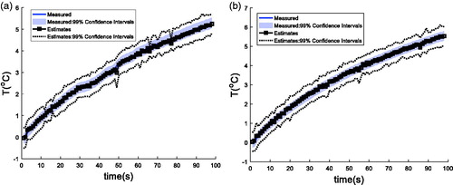
Figure 5(a) and (b) present the comparisons of the estimated and measured transient temperature variations at the position (r = 0, z = 8) mm, for the laser powers P₁ and P₂, respectively. These measurements were used for the solution of the state estimation problem. The associated 99% confidence intervals of the estimated and measured temperature variations are also included in these figures. It can be noticed in Figure 5(a) and (b) that the temperature variations estimated with the particle filter matched the measurements used for the solution of the state estimation problem, for both laser powers, at the graph scale. Note also the larger temperature variations observed for the larger power P₂ than for P₁.

Figure 5. Comparison of the measured and estimated transient temperature variations at (r = 0, z = 8) mm: (a) Laser power P₁; (b) Laser power P₂.

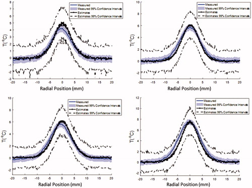
As a validation of the solution of the state estimation problem, the estimated temperature variations were compared to the measurements obtained with the thermocouple located at (r = 0, z = 10) mm, as well as with the temperature profiles at the heated surface. We note that these measurements were not used for the solution of the state estimation problem. Figures 6(a) and (b) present the comparison of the estimated temperature variations at the position (r = 0, z = 10) mm with the thermocouple measurements, for the laser powers P₁ and P₂, respectively. For both laser powers, the estimated mean temperatures fell within the measured 99% confidence intervals for most of the points. Maximum deviations between measurements and estimated means were 0.7 °C and 0.5 °C for P₁ and P₂, respectively. Figure 7 presents a comparison of the estimated radial temperature variations with the temperature measurements at the boundary exposed to the laser radiation (z = 0), at selected times (t = 60 s: top, t = 90 s: bottom), for the two laser powers (P₁: left, P₂: right). The measurements shown in Figure 7 were taken with the infra-red camera. The associated 99% confidence intervals of the estimated and measured temperatures are also included in this figure. As for the results presented above, Figure 7 shows that the temperature variations estimated with the proposed methodology were in excellent agreement with the measurements. Maximum deviation between measurements and estimated means was 0.8 °C. The measurements were obtained at pixels along a line drawn at the center of the phantom and clearly reveal the heating concentrated at the center of the phantom, where the laser beam was focussed. The measurements and the estimated temperatures assumed a Gaussian profile, due to the laser collimator used in the experiments and to the heat transfer process. Note in Figure 7 the larger temperature variations as time and laser power increase. This figure shows that the surface temperature spatial and transient variations were correctly estimated through the solution of the state estimation problem, with Liu and West’s version of the particle filter.

Figure 6. Comparison of the measured and estimated transient temperature variations at (r = 0, z = 10) mm: (a) Laser power P₁; (b) Laser power P₂.

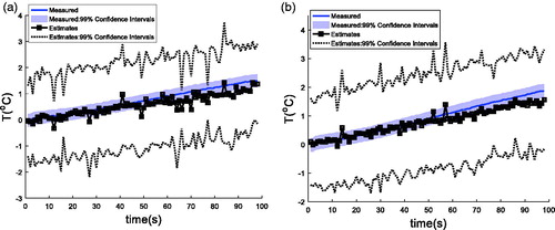
Figure 7. Comparison of the estimated radial temperature variation with the measurements obtained at z = 0 with an infra-red camera at selected times (t = 60 s: top; t = 90s: bottom). Experiment with P₁ (left) and P₂ (right).

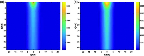
The temperature variation estimated in a longitudinal cut through the center of the phantom, at t = 90 s, is presented by Figure 8. This figure shows the highest temperatures in the region loaded with nanoparticles, which mimics the tumor. The distributions of fluence rates estimated on this same longitudinal cut are shown by Figure 9. This figure shows that, as expected, the estimated fluence rates were larger in the region of the laser beam and where the disk with nanoparticles was located. Moreover, the estimated fluence rates were larger for the highest laser power.

Figure 8. Estimated temperature variation on a longitudinal cut through the centre of the phantom at t = 90 s: (a) Laser power P₁; (b) Laser power P₂.

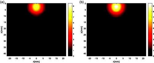
Figure 9. Estimated fluence rates on a longitudinal cut through the centre of the phantom at t = 90 s: (a) Laser power P₁; (b) Laser power P₂.

Besides the estimation of the state variables of interest for this problem, that is, the temperature and fluence rate fields, Liu and West’s algorithm of the particle filter allows for simultaneous estimation of the nondynamic model parameters. Figure 10 presents the estimated 99% confidence intervals for the model parameters, including the irradiances, for both P₁ and P₂. The means of the Gaussian priors used for each parameter are also shown by this figure. Figure 10 shows that the confidence intervals of the model parameters were sequentially reduced and tended to the mean values used for the priors, as the information provided by the measurements was taken into account in the solution of the state estimation problem. Moreover, the confidence intervals for the physical properties, which were estimated with the two different laser powers, were quite similar because these quantities are not functions of the incident irradiance. On the other hand, the confidence intervals of the irradiances tended towards the two different prior means, as these parameters were sequentially estimated for the two laser powers. The means and the 99% confidence intervals estimated for each parameter at the final time, t_f = 100 s, are presented by Table 3. In general, the prior means are within the estimated 99% confidence intervals, thus demonstrating the robustness of the present approach for simultaneous estimation of state variables and model parameters. Exceptions include the absorption coefficient of PVCP with nanoparticles, which was the parameter with the most uncertain prior (standard deviation of 10% of the prior mean). Similarly, the prior means for the absorption coefficient of PVCP and for the irradiance estimated with power P₂ are outside the estimated 99% confidence intervals, but still very close to their bounds. Maximum discrepancies between prior means and estimated means are of 4%, except for the absorption coefficient (10% for the power P₂).

Figure 10. Confidence intervals (99%) of the model parameters sequentially estimated with the particle filter: Experiments with P₁ (red) and P₂ (blue). Initial prior mean is shown by the grey line.

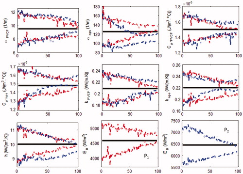
Table 3. Model parameters estimated at the final time t = 100 s.

			P1 = 156.6 mW		P2 = 220 mW
Parameter	Material	Prior Mean	Estimated Mean	Estimated 99% Confidence Interval	Estimated Mean	Estimated 99% Confidence Interval
k (W m^−1 K^–1)	PVCP	0.21	0.206	(0.201,0.211)	0.213	(0.206,0.219)
	PVCP with Fe2O3 NP	0.22	0.216	(0.209,0.222)	0.225	(0.216,0.234)
C (J m^−3 K^–1) × 10^–6	PVCP	1.4989	1.48	(1.46,1.50)	1.51	(1.46,1.56)
	PVCP with Fe2O3 NP	1.4755	1.50	(1.46,1.53)	1.54	(1.48,1.59)
κ (m^–1)	PVCP	9	9.2	(8.5,9.9)	9.7	(9.1,10.4)
	PVCP with Fe2O3 NP	125	133	(128,137)	113	(105,121)
h (W m^−2 K^–1)	—	10	10.1	(9.9,10.3)	9.8	(9.5,10.0)
E1 (Wm^–2)	—	4580.5	4645	(4519,4771)	—	—
E2 (Wm^–2)	—	6447.7	—	—	6282	(6162,6404)

Discussions

The estimation of the fluence rate and transient temperature fields, together with model parameters, was performed with Liu and West’s algorithm of the particle filter method [28], for a phantom heated by a laser diode. Transient measurements of one single thermocouple were used for the solution of the state estimation problem, in order to keep the number of intrusive sensors minimum, which is highly desirable for practical applications.

The results presented by Figure 5, where estimated and measured temperature variations are shown at the single measurement location used for the state estimation problem, demonstrates the accuracy of the particle filter technique applied in this work. The agreement between measurements and estimated temperatures was excellent, thus revealing quite small and uncorrelated residuals. The agreement between the estimated model parameters and those independently measured also reveals the accuracy of our solution. Indeed, despite the fact that priors with large variances were assigned to the model parameters, the maximum discrepancies between the prior means and the estimated means were of 2% for thermal conductivity and heat transfer coefficient, 4% for the volumetric heat capacity and 3% for the irradiance. The discrepancies ranged from 2 to 10% for the absorption coefficient, which was not independently measured in this work and involved the largest variances assumed for the prior. Therefore, the coupled mathematical model given by Equations (1)–(3), with the model parameters that were sequentially estimated together with the state variables (see Figure 10 and Table 3), were appropriate for the physical problem under analysis.

Temperature measurements, obtained with another thermocouple and with an infra-red camera, were used for the validation of the simultaneous estimation of state variables and model parameters. A comparison of the estimated temperatures and those measured by one thermocouple inside the phantom (in a region of small temperature variation), as well as those measured at the heated surface with the infra-red camera, are presented by Figures 6 and 7, respectively. These figures demonstrate the capabilities of the technique used in this work for predicting the temperature variations at locations where measurements were not used in the inverse analysis. Note in Figures 6 and 7 that both spatial and transient temperature variations were accurately estimated, with maximum discrepancies of 0.7 °C for internal temperatures and 0.8 °C for surface temperatures. Moreover, the estimated temperature distributions were physically meaningful, where the highest temperatures were estimated in the region of the disk loaded with the iron oxide nanoparticles that mimics a tumor (see Figure 8). Such a result is in accordance with the estimated fluence rate, which was higher in the region where the laser was incident (see Figure 9).

Differently from pure numerical simulation under uncertainty [43], the methodology used in this work naturally provides confidence intervals for the estimated quantities that reflect the amount of uncertainties present in the mathematical model and in the measurements. Besides the initial uncertainties of the parameters, which were represented by Gaussian priors, uncertainties related to the radiation and heat conduction models were also accounted for in the estimation procedure. Confidence intervals of the estimated quantities can be reduced by improving the prior beliefs on the parameters and on the models, for example, by performing other experiments. Moreover, the results could be further improved if additional sensors were used within the region of interest, because more information would be available for the estimation procedure [39]. On the other hand, we note in Figures 5, 6 and 7 that the estimated mean temperatures agreed with most of the measurements within the measurement uncertainties. Therefore, thermal damage to the tumor and healthy cells can be controlled with the temperatures estimated by the particle filter.

The temperature measurements required for the solution of the state estimation problem were intrusively obtained in this work with one thermocouple, since the experiments were conducted in a phantom. However, in practice they could have been taken with any other measurement technique. For example, synthetic magnetic resonance thermometry measurements were used for the solution of the state estimation problem in reference [11].

The iron oxide nanoparticles developed in this work concentrated the heating in the tumor region. Therefore, they might be quite effective in the hyperthermia treatment of cancer, by avoiding that healthy cells be unnecessarily exposed to high temperatures and thermally damaged.

The present work was focused on the validation of the solution of the state estimation problem in hyperthermia imposed by a laser diode. However, it can be readily extended to other heating methods, provided that the physical problem is appropriately modeled, as already demonstrated by the authors in earlier works for radiofrequency heating [15,17,18]. Furthermore, in our previous works the Pennes bioheat transfer model was used. Hence, the blood perfusion coefficient and the metabolic heat sources were treated as uncertain parameters and jointly estimated with other thermophysical properties and state variables, by using synthetic temperature measurements [13,17,18].

Conclusions

This work presented an experimental validation of the solution of a state estimation problem related to the hyperthermia treatment of cancer, by using a phantom. The phantom was manufactured with PVCP and contained a region loaded with iron oxide (Fe₂O₃) nanoparticles (24%vol). The nanoparticles (mean diameter of 10 nm) were manufactured during this work, for the hyperthermia experiments that used a laser diode in the near infra-red range (mean wavelength of 829.1 nm) as heat source. The state estimation problem was solved with Liu and West’s algorithm of the particle filter, which allowed for the simultaneous estimation of the model parameters and state variables.

Transient temperature measurements of one single thermocouple were used for the solution of the state estimation problem, resulting in quite small and uncorrelated residuals. Therefore, the mathematical model, with the parameters estimated via the particle filter, were appropriate for the physical problem under analysis. Moreover, the spatial and transient temperature variations that were estimated with the particle filter were validated, by using the temperature measurements of another thermocouple and of an infra-red camera. The temperature and fluence rate fields obtained with the solution of the state estimation problem revealed that the nanoparticles were effective in locally improving the absorption of the incident laser irradiance.

The results presented in this article demonstrated that the solution of the state estimation problem can be used to accurately obtain the temperatures in regions where measurements are not available. Therefore, the thermal damage to the tumor cells can be controlled for the sake of optimizing the hyperthermia treatment, while healthy cells are minimally affected by the temperature increase in the region.

Disclosure statement

No potential conflict of interest was reported by the authors.

Additional information

Funding

The authors are thankful for the support provided by Conselho Nacional de Desenvolvimento Científico e Tecnológico; Coordenação de Aperfeiçoamento de Pessoal de Nível Superior; Fundação Carlos Chagas Filho de Amparo à Pesquisa do Estado do Rio de Janeiro.

References

- Breasted JH. The Edwin Smith surgical papyrus: published in facsimile and hieroglyphic transliteration with translation and commentary. Univ. Chicago Orient. Inst. Publ. 1930. Available from http://trove.nla.gov.au/work/19048049%5Cnhttps://oi.uchicago.edu/research/pubs/catalog/oip/oip3.html%5Cnhttps://oi.uchicago.edu/research/pubs/catalog/oip/oip4.html%5Cnhttp://trove.nla.gov.au/version/41376704.
- Datta NR, Ordóñez SG, Gaipl US, et al. Local hyperthermia combined with radiotherapy and-/or chemotherapy: recent advances and promises for the future. Cancer Treat Rev. 2015;41:742–753.
- Mallory M, Gogineni E, Jones GC, et al. Therapeutic hyperthermia: The old, the new, and the upcoming. Crit Rev Oncol Hematol. 2016;97:56–64.
- Chatterjee DK, Diagaradjane P, Krishnan S. Nanoparticle-mediated hyperthermia in cancer therapy. Ther Deliv. 2011;2:1001–1014.
- Hirsch LR, Stafford RJ, Bankson JA, et al. Nanoshell-mediated near-infrared thermal therapy of tumors under magnetic resonance guidance. Proc Natl Acad Sci USA. 2003;100:13549–13554.
- El-Sayed IH, Huang X, El-Sayed MA. Surface plasmon resonance scattering and absorption of anti-EGFR antibody conjugated gold nanoparticles in cancer diagnostics: applications in oral cancer. Nano Lett. 2005;5:829–834.
- O'Neal DP, Hirsch LR, Halas NJ, et al. Photo-thermal tumor ablation in mice using near infrared-absorbing nanoparticles. Cancer Lett. 2004;209:171–176.
- Stafford RJ, Taylor BA. Practical clinical thermometry. In: Morose, E, editor. Physics of thermal therapy. Boca Raton (FL): CRC Press; 2013. pp. 41–52.
- Schena E, Tosi D, Saccomandi P, et al. Fiber optic sensors for temperature monitoring during thermal treatments: an overview. Sensors. 2016;16:1144.
- Winter L, Oberacker E, Paul K, et al. Magnetic resonance thermometry: methodology, pitfalls and practical solutions. Int J Hyperthermia. 2016;32:63–75.
- Pacheco CC, Orlande HRB, Colaço MJ, et al. State estimation problems in PRF-shift magnetic resonance thermometry. Int J Numer Methods. 2018;28:315–335.
- Notter M, Piazena H, Vaupel P. Hypofractionated re-irradiation of large-sized recurrent breast cancer with thermography-controlled, contact-free water-filtered infra-red-A hyperthermia: a retrospective study of 73 patients. Int J Hyperth. 2017;33:227–236.
- Lamien B, Orlande HRB, Eliçabe EG. Particle filter and approximation error model for state estimation in hyperthermia. J Heat Transfer. 2016;139:012001.
- Dos Santos I, Haemmerich D, Schutt D, et al. Probabilistic finite element analysis of radiofrequency liver ablation using the unscented transform. Phys Med Biol. 2009;54:627–640.
- Varon LAB, Orlande HRB, Eliçabe GE. Estimation of state variables in the hyperthermia therapy of cancer with heating imposed by radiofrequency electromagnetic waves. Int J Therm Sci. 2015;98:228–236.
- Lamien B, Orlande HRB, Eliçabe GE. Inverse problem in the hyperthermia therapy of cancer with laser heating and plasmonic nanoparticles. Inverse Probl Sci Eng. 2017;25:608–631.
- Varon LAB, Orlande HRB, Eliçabe GE. Combined parameter and state estimation in the radio frequency hyperthermia treatment of cancer. Numerical Heat Transfer, Part. A Aplicattions. 2016;70:581–594.
- Lamien B, Varon LAB, Orlande HRB, et al. State estimation in bioheat transfer: a comparison of particle filter algorithms. Int J Numer Methods. 2017;27:615–638.
- Dombrovsky LA, Timchenko V, Pathak C, et al. Radiative heating of superficial human tissues with the use of water-filtered infrared-A radiation: a computational modeling. Int J Heat Mass Transf. 2015;85:311–320.
- Paulides MM, Stauffer PR, Neufeld E, et al. Simulation techniques in hyperthermia treatment planning. Int J Hyperthermia. 2013;29:346–357.
- Pearce JA. Comparative analysis of mathematical models of cell death and thermal damage processes. Int J Hyperthermia. 2013;29:262–280.
- Robert CP, Doucet A, Andrieu C. Computational advances for and from Bayesian analysis. Stat Sci. 2004;19:118–127.
- Andrieu C, Doucet A, Singh SS, et al. Particle methods for change detection, system identification, and control. Proc IEEE. 2004;92:423–438.
- Arulampalam MS, Maskell S, Gordon N, et al. A tutorial on particle filters for online nonlinear/non-Gaussian Bayesian tracking. IEEE Trans Signal Process. 2002;50:174–188.
- Carpenter J, Clifford P, Fearnhead P. An improved particle filter for non-linear problems. IEE Proc Radar Sonar Navig. 1999;146:2.
- Doucet A, De Freitas N, Gordon N. Sequential Monte Carlo methods in practice. New York: Springer. 2001;178–195.
- Kantas N, Doucet A, Singh SS, et al. On particle methods for parameter estimation in state-space models. Stat Sci. 2015;30:328–351.
- Liu J, West M. Combined parameter and state estimation in simulation-based filtering. In: De Freitas JFG, Doucet, A, Gordon NJ, editors. Sequential Monte Carlo Methods in Practice. New York (NY): Springer-Verlag; 2001. pp. 197–223.
- Del Moral P, Doucet A, Jasra A. Sequential Monte Carlo samplers. J Royal Stat Soc B. 2006;68:411–436.
- Kihal A, Bouzabata B, Fillion G, et al. Magnetic and structural properties of nanocrystalline iron oxides. Physics Procedia. 2009;2:665–671.
- Mahadevan S, Gnanaprakash G, Philip J, et al. X-ray diffraction-based characterization of magnetite nanoparticles in presence of goethite and correlation with magnetic properties. Physica E Low Dimens Syst Nanostruct. 2007;39:20–25.
- Maybeck PS, Siouris GM. Stochastic models, estimation, and control, Volume I. IEEE Trans Syst Man Cybern. 1980;10:282–282.
- Kalman RE. A new approach to linear filtering and prediction problems. J Basic Eng. 1960;82:35.
- Kaipio JP, Fox C. The Bayesian framework for inverse problems in heat transfer. Heat Transf Eng. 2011;32:718–753.
- Rios MP, Lopes HF. The extended Liu and West filter: parameter learning in markov switching stochastic volatility models. State-sp. Model. Appl Econ Financ Stat Econ Financ. 2013;1:23–62.
- Sheinson DM, Niemi J, Meiring W. Comparison of the performance of particle filter algorithms applied to tracking of a disease epidemic. Math Biosci. 2014;255:21–32.
- Lopes HF, Carvalho CM, Online Bayesian learning in dynamic models: an illustrative introduction to particle methods. In: Damien P, Dellaportas P, Polson NG, et al. editors. Bayesian Theory Appl. Oxford University. Oxford, UK: Oxford University Press; 2013.
- Candy JV. Bayesian signal processing: classical, modern, and particle filtering methods. Class Mod Part Filter Methods. New York (NY): Wiley-Interscience; 2008.
- Orlande H, Colaço M, Dulikravich G, et al. State estimation problems in heat transfer. Int J Uncertain Quantif. 2012;2:239–258.
- West M. Approximating posterior distributions by mixture. J R Stat Soc Ser B. 1993;55:409–422.
- Fonseca M, Zeqiri B, Beard P, et al. Characterisation of a PVCP-based tissue-mimicking phantom for quantitative photoacoustic imaging. Proc SPIE Opto-Acoustic Methods Appl Biophotonics II. 2015;9539:953911.
- Jeong EJ, Song HW, Lee YJ, et al. Fabrication and characterization of PVCP human breast tissue-mimicking phantom for photoacoustic imaging. Biochip J. 2017;11:67–75.
- Fahrenholtz S, Stafford RJ, Maier F, et al. Generalized polynomial chaos based uncertainty quantification for planning MRgLITT procedures. Int J Hyperthermia. 2013;29:324–335.