In silico assessment of collateral eddy current heating in biocompatible implants subjected to magnetic hyperthermia treatments

Abstract

Purpose: Bearing partially or fully metallic passive implants represents an exclusion criterion for patients undergoing a magnetic hyperthermia procedure, but there are no specific studies backing this restrictive decision. This work assesses how the secondary magnetic field generated at the surface of two common types of prostheses affects the safety and efficiency of magnetic hyperthermia treatments of localized tumors. The paper also proposes the combination of a multi-criteria decision analysis and a graphical representation of calculated data as an initial screening during the preclinical risk assessment for each patient.

Materials and methods: Heating of a hip joint and a dental implant during the treatment of prostate, colorectal and head and neck tumors have been assessed considering different external field conditions and exposure times. The Maxwell equations including the secondary field produced by metallic prostheses have been solved numerically in a discretized computable human model. The heat exchange problem has been solved through a modified version of the Pennes' bioheat equation assuming a temperature dependency of blood perfusion and metabolic heat, i.e. thermorregulation. The degree of risk has been assessed using a risk index with parameters coming from custom graphs plotting the specific absorption rate (SAR) vs temperature increase, and coefficients derived from a multi-criteria decision analysis performed following the MACBETH approach.

Results: The comparison of two common biomaterials for passive implants - Ti6Al4V and CoCrMo - shows that both specific absorption rate (SAR) and local temperature increase are found to be higher for the hip prosthesis made by Ti6Al4V despite its lower electrical and thermal conductivity. By tracking the time evolution of temperature upon field application, it has been established that there is a 30 s delay between the time point for which the thermal equilibrium is reached at prostheses and tissues. Likewise, damage may appear in those tissues adjacent to the prostheses at initial stages of treatment, since recommended thermal thresholds are soon surpassed for higher field intensities. However, it has also been found that under some operational conditions the typical safety rule of staying below or attain a maximum temperature increase or SAR value is met.

Conclusion: The current exclusion criterion for implant-bearing patients in magnetic hyperthermia should be revised, since it may be too restrictive for a range of the typical field conditions used. Systematic in silico treatment planning using the proposed methodology after a well-focused diagnostic procedure can aid the clinical staff to find the appropriate limits for a safe treatment window.

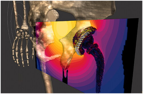
Graphical Abstract

Keywords:

• Magnetic hyperthermia
• eddy currents
• medical implants
• electromagnetic dosimetry
• in silico

1. Introduction

Magnetic hyperthermia has already been tested in clinical settings as an adjuvant to radiotherapy to successfully treat several types of tumors [1–3], especially glioblastoma multiforme. Beyond its use for inducing thermal damage and/or sensitizing tumors to first-line treatments, the heat implied in magnetic hyperthermia is also used to control the activation or the release of anticancer drugs [4,5] and to complement diagnostic techniques [6] into what is known as cancer theranostics, although these approaches are still a further step back from clinical studies due to the more complex regulatory process involved. The increase of more specialized instrumental development is relentless, and commercial systems are being deployed in Europe and USA; hence, research on safety, dosimetry and treatment planning should progress at the same pace. The therapy must be adapted to each patient and tumor, as well as to the evolution of the tumor throughout the process. In this regard, the development of virtual models of tumors from diagnostic data and the performance of computer simulations allow to improve the planning and execution of treatments and the predictions of the behavior of each tumor [7,8]. In the specific case of magnetic hyperthermia, the only data on simulations applied to clinical trials date back from the early 2000s [9–11]. These studies laid the foundations for treatment planning of magnetic hyperthermia in humans. In this context, the presence nearby the region of interest of passive irremovable metallic implants, like dental fillings, staples or orthopedic prostheses, constitutes an exclusion criterion in the available data on these clinical trials [12,13]. The core biomaterials for these implants are metallic or have metallic components – typically Ti6Al4V and, to a lesser extent since 2013, CoCrMo, due to some biocompatibility issues [14,15] – with electrical conductivity much higher than the one of the surrounding human tissues. These components, when exposed to the alternating magnetic fields (AMF), develop significant induced currents (eddy currents) that circulate mainly in proximity of their surface and create a secondary magnetic field counteracting the former. In addition, such eddy currents produce into the metallic components power dissipation (Joule losses), which translates into a temperature rise that diffuses to the surrounding tissues, leading to potential thermal damages [16]. This aspect is of particular interest given how often this kind of implants is found in prospective patients of the aforementioned techniques. Since only in the USA it was estimated that 7,2 million people were living with a joint implant back in 2014 [17], the probability of finding a prospective magnetic hyperthermia patient wearing a passive implant is relatively high. While receiving some attention in magnetic resonance imaging, for both radiofrequency and gradient coil signals [18–25], to date neither computational, nor experimental studies have been carried out on eddy current heating of implants as a side effect of magnetic hyperthermia treatments. Instead, up to now in the hyperthermia context the eddy current heating of implants comes from the use of some ferromagnetic electrodes or ‘thermal seeds’ (which could be here regarded as passive implants for the sake of comparison) that have been the active part of some other invasive hyperthermia modalities [26–28]. Perhaps, the lack of studies explains why the presence of metallic prostheses constitutes an exclusion criterion, as per the information available in relevant clinical trials registered in public databases [29].

As regards to direct thermal effects on native biological tissues, since 1998 the International Commission on Non-Ionizing Radiation Protection (ICNIRP) has recommended basic restrictions on the specific absorption rate (SAR), for frequency values above 100 kHz. Reference levels expressed in terms of unperturbed field quantities were established by ICNIRP as well [30].

These recommended thresholds have been questioned and revisited [31] due to the unclear implicit safety factors that may be preventing access to a wider range of field conditions in hyperthermia treatments. Certainly, the fact that higher frequencies (f) and magnetic field intensity (H) values could be employed, depending on the body region to treat, was pointed out by Stauffer et al. [32] and recognized by Atkinson et al. in their overall H·f threshold proposition [26].

The recently published 2020 ICNIRP Guidelines for Limiting Exposure to Electromagnetic Fields [33], which have updated the radiofrequency electromagnetic (EM) field part of the ICNIRP 1998 guidelines [30], and the 100 kHz to 10 MHz part of the ICNIRP (2010) low frequency guidelines [34,35] have defined new safety criteria and, consequently, new reference values. In particular, for occupational exposure the guidelines take a local SAR (i.e., specific absorption rate averaged over 10 g of contiguous tissue in every 6-min interval) in the head and torso of 10 W·kg⁻¹ as the local exposure level corresponding to the adverse thermal health effect threshold. Such a threshold is set to 5 °C for Type-1 tissues (e.g., fat, muscle, and bone) and to 2 °C for Type-2 tissues (e.g., all tissues in the head, abdomen, thorax, and pelvis not already included in Type-1). The SAR value already includes an appropriate safety factor to account for scientific uncertainty, as well as differences in thermal physiology across the population and variability in environmental conditions and physical activity levels.

Some methodology have been proposed to reduce tissue exposition to the external field in a study combining computer modeling and a proof-of-concept experimentation on a breast tumor phantom [36]. The proposed solution essentially comprises a coil displacement with respect to the tissues, aiming to control the formation of induced currents and consequently of hot spots, over the treated tissue. Although physically sound and feasible, these methods are still of limited application to deep-seated tumors due to the limited control on the field homogeneity over the region of interest and the required energy deposition to achieve a clinically effective heating. Besides, the influence on implants is yet to be studied.

The present work focuses on the collateral heating due to eddy currents induced in two largely prevalent categories of passive implants, dental implant and hip prosthesis, whose location typically matches that of some superficial tumors (head and neck) or deeper ones (prostate and colorectal). The obtained results question the current practice of considering implants as an exclusion criterion in clinical magnetic hyperthermia, since under many operational conditions the typical safety rule of staying below or attain a maximum temperature increase or SAR value is met, even considering the worst-case scenario. We propose the use of in silico treatment planning methods to assess the extent of eddy currents in passive implants and to evaluate whether or not they should be mitigated without compromising the field conditions needed for an effective therapy.

2. Materials and methods

Far from the tumor, the temperature increase induced by the exposure to the magnetic field is expected to be limited during a safe treatment. Hence, it should not be able to alter the electric properties of any relevant material significantly. Based on this assumption, the analysis of the eddy current heating of passive implants and surrounding tissues has been divided into two subsequent steps. First the electromagnetic problem is solved, to determine the eddy current distribution and power released. Then the thermal problem is studied to estimate the consequent temperature increase in tissues. In some case, the simulations predict a very large heating, which disproves the assumptions explained above. In such cases, the important point is that a potentially dangerous situation, which must be avoided, has been clearly found, even though the numerical value of the heating has a low accuracy.

In the electromagnetic problem, the interaction between the magnetic field generated by the sources (i.e., the coils used for the hyperthermia treatment) and any conductive medium (biological tissues and metallic objects) is studied by solving numerically the electromagnetic Maxwell equations. The secondary magnetic field H_i, generated by the currents induced in the radiated body, sums to the unperturbed source field H_s, giving rise to the total magnetic field H. Formally, this fact results in (1) $$\begin{array}{l}\text{curl}E=-{\mu }_0\frac{\partial H}{\partial t}\\ H=H_s+H_i\\ \text{curl}{H}_i=\sigma E\end{array}$$(1) where H(x,y,z,t) is the total magnetic field, function of the spatial coordinates x, y, z and the time t, E(x,y,z,t) is the induced electric field, σ is the local electrical conductivity, and μ₀ is the vacuum permeability. In low to medium frequency electromagnetic dosimetry (e.g., when the compliance with ICNIRP basic restrictions has to be verified to avoid unintentional nerve stimulation, from 1 Hz to 10 MHz), the secondary field can be disregarded when only native tissues are studied. This assumption is implemented in commercially available software for dosimetric analysis using highly detailed anatomical human models (e.g., Sim4Life [37]). However, in the presence of highly conducting elements (as the metallic implants), significant eddy currents produce secondary fields strong enough to alter the local magnetic field generated by the sources. This has a significant effect on the intensity and the spatial distribution of the eddy currents, and modifies the power deposition in the implant itself.

The presence of the secondary field H_i makes the numerical solution of Equation (1)(1) $$\begin{array}{l}\text{curl}E=-{\mu }_0\frac{\partial H}{\partial t}\\ H=H_s+H_i\\ \text{curl}{H}_i=\sigma E\end{array}$$(1) more complex with respect to the case when H_i is disregarded. In the adopted approach, the solution is obtained by introducing vector and scalar potentials as unknowns instead of the fields and by discretizing the resulting equations with a hybrid finite element–boundary element method (FEM–BEM) [38]. The problem is formulated in frequency domain, where the unknowns are phasors (complex quantities). The human model (with the inserted implant) is the computational domain discretized in voxels. Details of the numerical implementation are described in [38,39] and briefly recalled in the Supplementary Appendix A. The electromagnetic solver has been extensively tested by comparison with laboratory measurements on a phantom [40].

The second step of the procedure here adopted requires the solution of the thermal problem described by Pennes’ bioheat equation [41]: (2) $$\rho c_p\partial T/\partial t=\nabla \cdot \lambda \nabla T+h_b\left(T_b-T\right)+P_{\mathit{met}}+P_{em}$$(2) where ρc_p is the volumetric heat capacity, λ is the thermal conductivity, h_b is the blood perfusion coefficient in the human tissues, T_b is the temperature of blood, P_met is the volume power density associated with the metabolic process, and P_em is the volume power density dissipated within the metallic objects. The latter value is computed in each voxel of the implant, starting from the previous electromagnetic solution: $$P_{em}=\sigma {\left|\mathit{E}\right|}^2/2$$ being σ the electrical conductivity of the metal and E the peak value of the electric field. On the body surface (∂V, with outward normal unit vector n), Robin boundary conditions model the heat exchange with the external environment (supposed to be at the constant temperature T_air = 25 °C) Formally, by assuming a given heat exchange coefficient h_amb (h_amb ∼ 7 W/(m²·K)), this can be expressed as (3) $${\lambda \partial T/\partial n|}_{\partial V}=-h_{\mathit{amb}}\left(T-T_{\mathit{air}}\right)$$(3)

Thermoregulation processes are introduced in the thermal model by assuming that the perfusion coefficient h_b and the metabolic heat P_em are dependent on temperature, as proposed in [42]. Therefore, h_b = L_B h_b0, where L_B = is the local temperature-dependent multiplier (for T > T₀), being h_b0 the perfusion coefficient at the rest temperature T₀ and coefficient ΔB is set to 1.6 K. L_B was limited to 15 for all tissues except for skin, in which case the limit was 32. Analogously, P_met = L_met P_met0, being factor L_met = and P_met0 the metabolic heat at rest. This is an approximated model of the complex thermoregulation phenomena, which disregards the response times of the thermoregulatory process that regulates the core body and assumes an instantaneous regulation; in any case, it is considered appropriate for local temperature increase. It must be remarked that this model is valid for mild temperature increases, while it fails to represent the physiological behavior in the presence of strong heating and the related temperature increase. This consideration explains why the results for some combinations of implant and field intensity are not explicitely reported in the next tables.

The determination of the temperature evolution described by Equations (2)(2) $$\rho c_p\partial T/\partial t=\nabla \cdot \lambda \nabla T+h_b\left(T_b-T\right)+P_{\mathit{met}}+P_{em}$$(2) and (3)(3) $${\lambda \partial T/\partial n|}_{\partial V}=-h_{\mathit{amb}}\left(T-T_{\mathit{air}}\right)$$(3) requires the knowledge of the spatial distribution of the temperature before the electromagnetic exposure (T₀), determined by the metabolic heat and the diffusion-perfusion phenomena, and the temperature of blood (T_b). Since we are interested in the temperature elevation caused by the exposure to an electromagnetic field, the thermal problem is here handled by introducing the temperature elevation ΔT with respect to T₀ as unknown (ΔT = T - T₀), so that the problem can be rewritten as (4) $$\mathrm{\rho }{c}_{\mathrm{p}}\partial \left(\mathrm{\Delta }T\right)/\partial t=\nabla ·\left[\mathrm{\lambda }\nabla \left(\mathrm{\Delta }T\right)\right]-2^{\mathrm{\Delta }T/\mathrm{\Delta }B}{h}_{\mathrm{b}0}\mathrm{\Delta }T+\left({1.1}^{\mathrm{\Delta }T}-1\right)P_{\mathrm{met}0}+P_{\mathrm{em}}$$(4) with Robin boundary conditions $${\lambda \partial \left(\Delta T\right)/\partial n|}_{\partial V}=-h_{\mathit{amb}}\left(\Delta T\right).$$

The thermal problem (Equation 4(4) $$\mathrm{\rho }{c}_{\mathrm{p}}\partial \left(\mathrm{\Delta }T\right)/\partial t=\nabla ·\left[\mathrm{\lambda }\nabla \left(\mathrm{\Delta }T\right)\right]-2^{\mathrm{\Delta }T/\mathrm{\Delta }B}{h}_{\mathrm{b}0}\mathrm{\Delta }T+\left({1.1}^{\mathrm{\Delta }T}-1\right)P_{\mathrm{met}0}+P_{\mathrm{em}}$$(4) ) is solved by a finite difference method (FDM) using Douglas–Gunn (DG) time split scheme in a domain including both the implant and the human body. The characteristics of the DG algorithm allow a parallel implementation on GPUs. Details of the numerical implementation can be found in [24], together with its validation in comparison with Semcad X software.

The numerical simulations were carried out using the ‘Duke’ model, a high-resolution healthy male human model developed by the IT’IS Foundation [43] as part of the Virtual Family computational models [44]. The original version of this model includes about 80 different tissues, whose electric and thermal properties have been set according to the database of the IT’IS Foundation [45,46]. As discussed in Supplementary Appendix B, the computational domain is limited to a suitable portion of the human model, by taking advantage of the local nature of the heating induced by the dissipated power into the metallic objects. A wide range of passive implants can be encountered in the clinical environment and could be suitable for this study. From all the possible designs and purposes, two exemplary kinds of prostheses were selected: a hip prosthesis for total joint replacement and a dental implant used to supply the absence of a dental piece. These two implants were chosen due to their high prevalence and to their location in the body. The first one is placed in an inner part of the body, considering it a deep-seated prosthesis, whereas the dental implant is found in a superficial area of the head, making it a shallow prosthesis. For the hip implant study, the human model was truncated including both hips with height from the anterior inferior iliac spine to 15 cm downwards from the greater trochanter, leaving the prosthesis centered in the z axis. In the simulations involving the dental implant, the human phantom included the head and the neck up to the height of the T2 vertebra. The shoulders were cut off following the midclavicular line on both sides.

The 3 D models of the investigated implants were placed inside the healthy human model Duke in their anatomical positions. Both prosthesis models were downloaded from GRABCAD community [46,47] and adapted to the human model using the open source 3 D creation suite Blender [48] to reproduce, as close as possible, the real clinical situation. This adjustment consisted on minimal deformations in small areas of the implant models to avoid some undesired overlapping between the tissues and the inserted objects without losing its original design.

The hip model was placed in the right femur. The model of this bone was also modified mimicking how it is sectioned during a total hip replacement surgery, where the head of the femur is cut and the stem of the implant is introduced inside the bone.

For the dental implant, the procedure was simpler, since the implant consists of a screw that is introduced in the bone once the dental alveolus is naturally occupied again with new bone tissue. To virtually reproduce this process, the socket in the mandibular bone that corresponds to the dental piece 36 was filled with cortical bone. The roots of the piece were cut and the remaining part was used as a model for the ceramic crown for the implant. The screw of the prosthesis was placed in the bone by overlapping it to the models.

In order to check the idea that the position of the coil with respect to the metallic part is crucial to decide whether the therapy is safe or not for a specific patient, the electromagnetic field was studied placing the source in three different regions of the human model. Two of them were the two clinical cases explained before. In a third scenario, that we have defined as the ‘worst-case scenario,’ the coil was placed as close as possible to the prosthesis.

The field applicator considered for the hip prosthesis simulations is a generic flat, round, multiturn (often referred as ‘pancake’) coil, which has been placed in front of the areas where theoretical colon and prostate tumors might be. The applicator can impose a magnetic flux density of about 5 mT, 10 mT or 15 mT in the area where these lesions would be treated. However, given the linearity of the governing equations of the electromagnetic model, the results obtained in this way can be scaled, quadratically, to any amplitude adopted during interventions, provided that thermoregulation processes are disregarded. Even though the worst-case scenario is an improbable setup in the clinical environment, it will help us to better understand how the variation of the field reaching the prosthesis depends on the coil position. For this comparison, the set of field intensity values tested in the three cases were 5 mT, 10 mT and 15 mT at the theoretical tumor considered in each case. Besides safety reasons, these field intensity values have been chosen considering the experimental conditions met in numerous in vitro and in vivo studies [49,50]. In particular, most of the magnetic colloids intended for magnetic hyperthermia usually heat above 43 °C for intensities below 30 mT and frequencies within 100–300 kHz for variable application times [49].

The field applicator considered for the dental implant is a 3-turn open collar-type coil adapted to the shape of the patient’s neck. Unlike other non-portable devices approved for use in humans [51], these generic field applicators are as portable as those considered for ongoing clinical trials [52]. The main advantage of this type of coils is that the field is projected over the patient and can be adapted to virtually any region. Only one position of the coil has been considered, assuming a 5 mT, 10 mT and 15 mT magnetic flux density in the neck, specifically in the region where a superficial tumor would be located. It is expected that patients bearing a dental implant will also have a metal ceramic crown screwed to it to make up for the lack of the dental piece. Since this partially metallic object can be easily removed, both cases with and without crown have been compared.

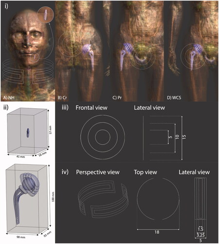
Figure 1 shows the hip and dental prostheses included inside the human model together with the position of the field applicator for neck, colon, prostate and worst-case scenario, from left to right. In this figure, the implants are also presented with the test volumes where the analyses are performed and a detailed description of the coils used as applicators is provided.

Figure 1. (i) Virtual models used for each of the considered cases, indicating the position of prostheses and coils (white hairlines): (a) head-and-neck, (b) colorectal, (c) prostate, and (d) worst-case scenario tumor locations. For (a) a 3-turn open collar-type coil has been considered, while for (b), (c) and (d) a 3-turn (inner turn of 5 cm, intermediate turn 10 cm, and outer turn of 15 cm) non-spiral, single layer, flat air coil has been used instead. For comparison purposes, prostheses are made of either Ti6Al4V or CoCrMo alloys in all the indications. (ii) Portion of voxels in the surrounding of each prosthesis that are taken into account for the scatter plot analysis. (iii) Detail of the coil used for CR, Pr and WCS tumor locations. Dimensions are presented in mm. (iv) Detail of the coil used for NH tumor location. Dimensions are presented in mm.

The resulting model of a patient carrying the implants were discretized with cubic voxels following a homogeneous grid with spatial resolution 2 mm × 2 mm × 2 mm for the hip prosthesis and 0.5 mm × 0.5 mm × 0.5 mm in the case of the dental implant. The stability of the results was preliminarily verified by increasing the spatial discretization until the unavoidable error in the approximated total power is considered acceptable, according to the approach presented in [53], where an experimental comparison was available. Further information about gridding can be found in Supplementary Appendix B, where the approach adopted to face the problem of the ‘skin effect’ in metals is also described.

The present study considers two of the most common alloys used in hip prosthesis (CoCrMo and Ti6Al4V), which have excellent mechanical characteristics [54]. The same titanium alloy was adopted for the dental screw, while a typical metal-ceramic used in dental prosthetics was the crown material. Electrical and thermal properties of the adopted materials are summarized in Table 1.

Table 1. Electrical and thermal properties of the implant materials used in the simulations.

Material	$\sigma \mathrm{ }(\mathrm{kS}/\mathrm{m})$	$\rho \mathrm{ }(\mathrm{kg}/{\mathrm{m}}^3)$	$c_p\mathrm{ }(\mathrm{J}/(\mathrm{kg}·\mathrm{K}))$	$\lambda (\mathrm{W}/(\mathrm{m}·\mathrm{K}))$
Ti6Al4V [55]	560	4430	526.3	6.7
Metal-ceramic [56,57]	0.16	8400	450	13
CoCrMo [57]	1160	8400	450	13

The analysis was always performed assuming sinusoidal supply conditions at the frequency of 300 kHz, within the range intended for hyperthermia treatments. About this, it must be pointed out that the skin effect occurring in metallic components with high electric conductivity can alter the quadratic dependence of the energy deposited in the tissue by the AMF on the frequency and therefore the overall proposed H·f threshold is no longer rigorously valid. Thus, the results here presented are valid for a frequency range of around 300 kHz, but cannot be straightforwardly extended to considerably different frequency values.

Finally, the software M-MACBETH [58] was used to perform the Measuring Attractiveness by a Categorical Based Evaluation Technique (MACBETH) to evaluate the coefficients of the risk index equation described in section 3.1 (further information can be found in Supplementary Appendix C).

3. Results

3.1. Sar vs ΔT log-log graphs

There is still debate on whether SAR or temperature should be used as a metric for dosimetry and in which cases. Many estimations have been done so far on a possible relationship between SAR and temperature (see for example [59,60]), mainly in the megahertz–gigahertz frequency range, more specifically with reference to magnetic resonance imaging and other hyperthermia modalities . This correlation has been barely studied in the kilohertz range [61] and deserves immediate attention for medical technology operating in that frequency range, not only for magnetic hyperthermia, but also for other next-generation techniques like magnetic particle imaging [62,63].

In the present work, two quantities were assumed as safety indicators: the distributions of both SAR and temperature increase (ΔT) evaluated after 5 and 30 min of continuous exposition in a test volume around the prosthesis. The tested volume for both kinds of prostheses is the portion of parallelepiped shown in Figure 1(ii) where the volumes taken up by the implants have been removed. The boundaries of the test volumes are chosen so that no variation of the externally applied field with the secondary field generated by the eddy currents in the prosthesis is observed. For the resulting representation (Figures 2 and 4 and figures in Supplementary Appendix D), each tissue voxel (excluding the implant voxels) belonging to the test region is associated with the couple of corresponding values of SAR and ΔT and displayed in a log-log graph with ΔT as abscissa and SAR as ordinate. The scatter plots are divided into four quadrants by the vertical and horizontal lines. The horizontal line is associated with the safety thresholds for SAR, which is 10 W/kg assuming for patients the same basic restriction on local SAR defined in ICNIRP 2020 for occupational exposure. The vertical line is associated with the threshold ΔT = 5 °C according to ICNIRP 2020 guidelines [33] to set basic restrictions against thermal effects of electromagnetic exposure. The corresponding graphs considering 1 °C as ΔT threshold following IEEE recommendations [64,65] can be found in [66].

Figure 2. Log-log scatter plots of ΔT versus SAR for bone voxels at f = 300 kHz with magnetic flux density of 15 mT without accounting for thermoregulation. The figures in the right column refer to colon tumor, the one in the left column to prostate tumor. Color varies depending on the distance of each voxel to its closest point in the coil (reddish points are closer to the coil and bluish points are farther from it). The thresholds are established according to ICNIRP 2020 guidelines for type 1 tissues, namely ΔT = 5 °C and SAR = 10 W/kg.

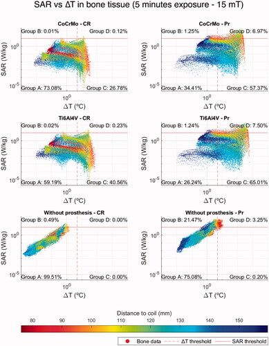
The first quadrant A (lower left) of the SAR vs ΔT scatter plots (Figure 2) includes the voxels whose values are below the aforementioned SAR and ΔT thresholds, thus, satisfying the recommendations done by ICNIRP/IEEE for electromagnetic field exposures of living beings. The second quadrant B (upper left) contains the voxels where SAR values overcome the safety limit (SAR ‘hot spots’), but, because of the effects of blood perfusion and diffusion parameters, the temperature rise remains below the threshold. It is known that high SAR values do not necessarily imply a high biological effect; moreover, low SAR values may have larger biological effects than higher ones in certain cases [67]. Consequently, quadrant B may also contain voxels of tissues bearing a low hazard potential despite their high SAR values. The voxels in the third quadrant C (lower right) show SAR values below the threshold, but overcome the limit established for the temperature increase. Most of the voxels in this quadrant move back to the first one A when the simulations are carried out without prostheses. Since the low SAR values do not justify in itself the temperature increase, the warming of these voxels can be attributed to the heat produced in the metallic components of the prostheses and diffused in the surrounding tissues. In order to validate this hypothesis, a simple verification based on two steps simulations was prepared. The thermal problem was solved twice, first nullifying the SAR values of the tissue voxels (solution 1), and successively nullifying the electromagnetic power dissipated in the prosthesis voxels (solution 2). These results are finally compared against the complete simulation. The comparison confirmed the previous hypothesis, showing that the highest contribution in ΔT comes from the heat produced in the prosthesis and diffused in the surrounding tissues. Further information regarding these solutions can be found in Supplementary Appendix E. Finally, the last quadrant D (upper right), collects the voxels where both SAR and ΔT thresholds are trespassed.

Additionally, a table shows the percentage of voxels belonging to each quadrant. This compact quantitative representation of the results can be used as a simplified version of some of the most common multivariate decision tools adopted in the clinical environment [68]. We propose a set of parameters according to the risk inherent to each quadrant due to the different physiological effects depending on the range of temperature increase [69]. A rough risk index, but sufficient for the aim of this study, is obtained by combining these parameters with the voxel distribution into the quadrants, as in the following Equation (5)(5) $$\text{risk index}=0.0555·\mathrm{A}+0.1165·\mathrm{B}+0.4439·\mathrm{C}+0.5199·\mathrm{D},$$(5) : (5) $$\text{risk index}=0.0555·\mathrm{A}+0.1165·\mathrm{B}+0.4439·\mathrm{C}+0.5199·\mathrm{D},$$(5) being A, B, C and D the percentage of voxels in the corresponding quadrant. The numerical coefficients multiplying A, B, C and D are decimal fractions derived from a multi-criteria decision analysis (MCDA) that is described in Supplementary Appendix C. For the present case we have adopted the Measuring Attractiveness by a Categorical Based Evaluation Technique (MACBETH) [70], which is a pairwise comparisons method aimed to judge the difference of attractiveness between different options (the quadrants of the proposed SAR vs ΔT log-log graphs) using a set of relevant criteria. The latter were partially based on similar analysis made on drugs for treating metastatic cancers [71,72], on the current ICNIRP guidelines [33], on evidences from in vitro and in vivo testing of thermal damage [73–75] and also on the available clinical data on magnetic hyperthermia treatments of prostate cancer [1,2,76].

The scatter plots and the associated table to each plot are found to be a useful tool to quickly estimate the harmful potential of each treatment situation, able to put in evidence the presence of excess power deposition (i.e., SAR and ΔT hot spots), which cannot be evaluated only considering the whole-body SAR. Each risk index is associated to a color tag which corresponds to a range determining the severity of the situation. These ranges are: a) Safe (S) in green with risk index <0.1; b) Acceptable (A) in yellow with risk index ≥0.1 and <0.15; c) Risky (R) in red with risk index ≥0.15 and <0.3, and d) Very Risky (VR) with risk index ≥0.3. The thresholds have been chosen considering the literature on similar indications and general effects of heat on tissues [73–76].

3.2. Analysis of the hip prosthesis

The results obtained in the evaluation of the effects produced in bone tissue within the control volume around a hip prosthesis, considering both colon and prostate scenarios and both materials (CoCrMo and Ti6Al4V alloys), are presented in Figure 2, Supplementary Figures S3 and S4 and Table 2 in comparison with the case without prosthesis. Here, the temperature increases were estimated neglecting the thermoregulatory effects (i.e., hyperemia or vasodilation, variation of metabolic heating, sweating [77]). After 5 min of exposure, extremely large temperature increases (over 30 °C) are already observed.

Table 2. Percentage of bone tissue voxels that land in each quadrant for fields of 5, 10 and 15 mT in the tumor region for each case for both 5- and 30-min exposure.

		5 min exposure					30 min exposure
		Quadrant				Risk	Quadrant
		A	B	C	D		A	B	C	D	Risk
5 mT	CR CoCrMo	100.00%	0.00%	0.00%	0.00%	0.06 (S)	99.21%	0.00%	0.79%	0.00%	0.06 (S)
	CR Ti6Al4V	99.27%	0.00%	0.73%	0.00%	0.06 (S)	95.58%	0.00%	4.42%	0.00%	0.07 (S)
	CR without prosthesis	100.00%	0.00%	0.00%	0.00%	0.06 (S)	100.00%	0.00%	0.00%	0.00%	0.06 (S)
	Pr CoCrMo	78.61%	0.00%	21.17%	0.22%	0.14 (A)	71.69%	0.00%	28.09%	0.22%	0.17 (R)
	Pr Ti6Al4V	82.11%	0.00%	17.63%	0.26%	0.13 (A)	Out of range	Out of range	Out of range	Out of range	Out of range
	Pr without prosthesis	99.99%	0.01%	0.00%	0.00%	0.06 (S)	99.99%	0.01%	0.00%	0.00%	0.06 (S)
10 mT	CR CoCrMo	90.15%	0.00%	9.84%	0.00%	0.09 (S)	80.68%	0.00%	19.31%	0.00%	0.13 (A)
	CR Ti6Al4V	82.03%	0.00%	17.95%	0.02%	0.13 (A)	75.89%	0.00%	24.09%	0.02%	0.15 (R)
	CR without prosthesis	99.94%	0.06%	0.00%	0.00%	0.06 (S)	99.94%	0.06%	0.00%	0.00%	0.06 (S)
	Pr CoCrMo	Out of range	Out of range	Out of range	Out of range	Out of range	Out of range	Out of range	Out of range	Out of range	Out of range
	Pr Ti6Al4V	Out of range	Out of range	Out of range	Out of range	Out of range	Out of range	Out of range	Out of range	Out of range	Out of range
	Pr without prosthesis	87.73%	12.27%	0.00%	0.00%	0.06 (S)	87.73%	12.27%	0.00%	0.00%	0.06 (S)
15 mT	CR CoCrMo	75.60%	0.02%	24.25%	0.14%	0.15 (R)	67.71%	0.02%	32.13%	0.14%	0.18 (R)
	CR Ti6Al4V	68.73%	0.04%	30.99%	0.25%	0.18 (R)	63.29%	0.04%	36.43%	0.25%	0.20 (R)
	CR without prosthesis	99.47%	0.53%	0.00%	0.00%	0.06 (S)	99.47%	0.53%	0.00%	0.00%	0.06 (S)
	Pr CoCrMo	Out of range	Out of range	Out of range	Out of range	Out of range	Out of range	Out of range	Out of range	Out of range	Out of range
	Pr Ti6Al4V	Out of range	Out of range	Out of range	Out of range	Out of range	Out of range	Out of range	Out of range	Out of range	Out of range
	Pr without prosthesis	Out of range	Out of range	Out of range	Out of range	Out of range	Out of range	Out of range	Out of range	Out of range	Out of range

Risk column color indicates the safety of each case according to Equation (5)(5) $$\text{risk index}=0.0555·\mathrm{A}+0.1165·\mathrm{B}+0.4439·\mathrm{C}+0.5199·\mathrm{D},$$(5) , the darker, the riskier; and a letter that indicates the risk: (S), safe; (A), acceptable; (R), risky; (VR), very risky. Note that results presented for Pr Ti6AlV at 5 mT shown in bold italics are after 2 min exposure instead of 5. This corresponds to the last instant the thermoregulation model retrieves.

The data obtained from the colorectal simulations without thermoregulation were compared with the results obtained accounting for thermoregulation under the same magnetic flux densities: 5 mT, 10 mT and 15 mT (Supplementary Figure S3). This comparison showed that the thermoregulatory effects reduce the temperature increase. In the colon case, the maximum temperature rise in bone tissue drops from 77.68 °C to 60.85 °C in the Ti6Al4V hip implant and from 37.10 °C to 35.12 °C in the CoCrMo prosthesis under a 15 mT field. For simulations in the prostate case, the adopted numerical solver of the non-linear thermal problem required a too fine time discretization to provide a good approximation of the temperature increase. The data corresponding to these simulations are shown in Table 2 and Supplementary Table S7 as ‘Out of range.’ On the other hand, the heating predicted for prostate simulations without thermoregulation is very large and, as mentioned in Section 2, disproves a posteriori the assumptions at the foundation of the computational scheme. Nevertheless, the obtained results are still relevant, because high temperatures, and therefore unsafe conditions, are undoubtedly identified. Further information regarding other relevant tissues in the hip test volume, such as fat and muscle, are presented in Supplementary Appendix D, Tables S8 and S9 and in Ref. [66].

The calculated data reveal how the presence of the hip implant always enhances the risk for the patients. The number of voxels belonging to the ‘safe’ quadrant A significantly reduces for the major tissues studied, mainly for the bone, which is in intimate contact the metallic object. This result, although it cannot be generalized since it is limited to the adopted conditions, seems to partially justify the exclusion criterion for the patient with metallic prosthesis in most, but not all, cases. For example, the colon case at the lowest magnetic flux density after 5 min of continuous exposure appears to be safe in all tissues, even neglecting thermoregulation, whether the prosthesis is present or not, regardless of the biomaterial chosen. On the contrary, for the prostate treatment the presence of the prosthesis has to be handled with caution even at the lowest field intensity, especially at bone level. Furthermore, this is also shown in the data obtained from the thermoregulation model after 30 min exposure also for a magnetic field of 5 mT (Supplementary Figure S3(b)). Nevertheless, although ΔT increases always with the presence of a prosthesis, it is central to work out whether this effect may produce an irreversible damage to the patient beyond the reported discomfort caused by a temperature increase [2]. For such a purpose, the proposed coupled plot-table can play a key role in multivariate decision trees to conclude if the therapy is safe: being complemented, among others, with CEM43 estimators and thermoregulatory tissue effects, which were not considered in some cases due to the range of applicability of the applied thermoregulation model when solving the heat exchange problem. This implies that ΔT has been overestimated in some of these analyses, for instance, in the prostate case. The physiological effects due to heat generated along the exposure time also have to be addressed according to its threshold for thermal damage [73]. This will verify if the extreme temperature values reached in a particular tissue implies temporary, permanent or no damage at all.

The analysis puts in evidence that in all situations with and without prosthesis, the field application related to the prostate tumor may lead to the occurrence of some thermal hot spots also without metallic parts. The relative low distance from the field source explains this result, shown in the plots as a concentration of red dots in the upper-rightmost region of the cloud of points.

For the colon case, the SAR limit is rarely exceeded, even if hazardous temperature increases take place. For the three field intensities, the majority of points in quadrant C show middle distances to the coil, confirming that the calculated ΔT for these voxels is due to heat diffusion from the prosthesis. In addition, there are not large differences between the SAR value distributions with and without prosthesis proving that the heat increase is not due to the direct power deposition in the tissue.

Even if the shape of the voxel distributions in the SAR – ΔT –plane is similar for the two alloys, both SAR and ΔT are found to be higher for the hip prosthesis made by Ti6Al4V with respect to the ones of CoCrMo, even if the electrical conductivity of the titanium alloy is about one half of that of CoCrMo. Such a behavior, which may appear as surprising, occurs in high conductivity materials when the skin effect becomes relevant. This aspect is discussed in more detail and justified in Supplementary Appendix F using a simplified model problem.

3.3. Analysis of the source position with respect to the hip prosthesis

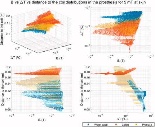
The outcome of the previous analysis for the colon and prostate cases was scaled to have the same field intensity equal to 5 mT in the closest area of the skin to the source. Since SAR, strictly speaking, is defined in biological tissues only, in the scatter plots, which include only the prosthesis voxels, the magnetic flux density B was used instead. The ΔT-B relationship was complemented with the minimum distance to the source, obtaining a 3 D scatter plot. Figure 3 shows the 3 D scatter plot for the prosthesis made of Ti6Al4V, comparing the results of the treatment of colon and prostate tumors with the ones of the worst-case scenario, where the highest B values are expected due to its proximity to the field source. As can be seen, if the source is placed far enough from the implant while guaranteeing a sufficient H at the region to treat, the probability of achieving a treatment within the safety standards for thermal therapies is much higher.

Figure 3. Different views of the 3 D scatter plot of the magnetic flux density through the prosthesis voxels, the increment of temperature for these voxels and the closest distance to the coil for the three cases studied: (a) 3 D view, (b) XY view, (c) XZ view, and (d) YZ view.

3.4. Analysis of the dental implant

The effects of the dental implant on the bone tissue, the closest to the implant, after a continuous exposure of 30 min are presented in Figure 4 and Table 3 following the same procedure as for the hip prosthesis. For this analysis, only a magnetic flux density value of 15 mT in the neck region was applied, accounting for the thermoregulation effects. This data gives an evaluation of the impact due to the presence of the metal ceramic crown.

Figure 4. Log-log scatter plots representing the ΔT and SAR of bone voxels for a dental implant studied with and without the metal-ceramic crown attached to it both exposed for 30 min to the same applied ac field with f = 300 kHz and 15 mT. The thresholds are established according to ICNIRP 2020 guidelines for type 1 tissues, namely ΔT = 5 °C and SAR = 10 W/kg.

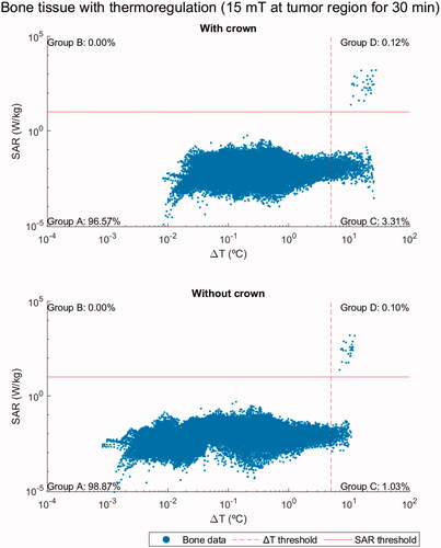
Table 3. Percentage of bone tissue voxels that fall within each quadrant in Figures 4, Supplementary Figures S5 and S6 plots.

				Quadrant				Risk
				A	B	C	D
With thermoregulation	5 min exposure	5 mT	With crown	99.90%	0.10%	0.00%	0.00%	0.06 (S)
			Without crown	99.92%	0.08%	0.00%	0.00%	0.06 (S)
		10 mT	With crown	98.83%	0.00%	1.05%	0.12%	0.06 (S)
			Without crown	99.88%	0.04%	0.02%	0.06%	0.06 (S)
		15 mT	With crown	97.03%	0.00%	2.85%	0.12%	0.07 (S)
			Without crown	98.95%	0.00%	0.95%	0.10%	0.06 (S)
	30 min exposure	5 mT	With crown	99.99%	0.01%	0.00%	0.00%	0.06 (S)
			Without crown	99.99%	0.01%	0.00%	0.00%	0.06 (S)
		10 mT	With crown	98.62%	0.00%	1.26%	0.12%	0.06 (S)
			Without crown	99.86%	0.03%	0.04%	0.06%	0.06 (S)
		15 mT	With crown	96.57%	0.00%	3.31%	0.12%	0.07 (S)
			Without crown	98.87%	0.00%	1.03%	0.10%	0.06 (S)
Without thermoregulation	5 min exposure	5 mT	With crown	99.90%	0.10%	0.00%	0.00%	0.06 (S)
			Without crown	99.92%	0.08%	0.00%	0.00%	0.06 (S)
		10 mT	With crown	96.91%	0.00%	2.97%	0.12%	0.07 (S)
			Without crown	99.65%	0.02%	0.26%	0.07%	0.06 (S)
		15 mT	With crown	91.86%	0.00%	8.02%	0.12%	0.09 (S)
			Without crown	97.40%	0.00%	2.51%	0.10%	0.07 (S)

Risk column color indicates the safety of each case according to expression (5), the darker, the riskier; and a letter that indicates the risk: (S), safe; (A), acceptable; (R), risky; (VR), very risky.

Table 3 clearly shows the improvement on the safety parameters considered when the metal ceramic crown is removed. Indeed, the shielding effect of the ceramic coating of the crown produces a temperature increase within the implant, and therefore, in the surrounding tissues. In some points, especially when the crown is not removed, the SAR threshold is exceeded. Despite these risky points, the percentage of bone voxels in potentially unsafe quadrants is very low (above 90% are in quadrant A in all the cases studied) in comparison with the results for the hip. Moreover, this scenario for dental implant is much less critical than the two other clinical treatments analyzed above, even though the magnetic flux density is similar to the case of the hip prosthesis for the same ac field setup. This suggests that the volume of the metallic part significantly influences the safety of treatment. Further information about these results can be found in Supplementary Figures S5, S6 and Table S10 and in Ref. [66].

3.5. Influence of prostheses on the treated region

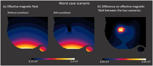
The significant eddy currents induced in metallic objects generate a secondary magnetic field that could distort the effective field produced by the applicator in the tissues as well as in the nanoparticles under the hyperthermia treatment. In order to verify how this alteration could affect the treatment efficacy, the effective magnetic field distributions in the radiated region with and without the prosthesis are compared in Figure 5(a). This study was performed for the Ti6Al4V hip prosthesis in the worst-case scenario, where the most intense secondary field is expected because the distance between coil and prosthesis is the shortest and the power deposition is the highest. The ac field applied was set up for f = 300 kHz and 5 mT at the skin level. The comparison shows that the highest differences are localized in a limited space very near to the prosthesis and drop very fast with the distance (Figure 5(b)), without affecting the region under treatment. The field variation starts to be negligible 1–2 cm away from the metallic surface and reaches a maximum intensity of 1 mT in the area closest to the surface of the prosthesis. As a rule of thumb, the secondary field produced by eddy currents should not affect the hyperthermia treatment – with the exception of the hypothetical case where the tumor, and hence the injected nanoparticles, were in close contact with the prosthesis.

Figure 5. Slice Z normal views: (a) of the effective magnetic field for the worst-case scenario with and without prosthesis for an ac field with 5 mT at skin level; and (b) of the difference between effective magnetic field for the worst-case scenario with and without Ti6Al4V prosthesis. The alteration due to the generated field drops to values around 0.1 mT for distances below 1 cm away from the implant.

Since the magnetic field intensity decays as the distance to the source increases, SAR in tissues will also decrease and, consequently, so will do ΔT. In order to minimize undesired effects, the easiest ways would seem a change of the source position. However, if the coil is just moved farther from the region of interest, the field intensity of the source has to be increased to guarantee a sufficient heating up of the nanoparticles at the tumor site. By doing so, a wider area would become exposed to a more homogenous field. If the source is far enough, the field applied in the surrounding area could reach an intensity close to the one of the treatment region, so too high to be safe in the presence of a metallic implant. As the displacement of the source might not be a solution in some cases, other strategies should be studied, such as diverse coil designs or different field intensity and frequency pair values, for instance.

Besides knowing the absolute maximum temperatures that are reached in the different tissues, it is also important to know the rate at which these values are attained during the treatment. This information allows an adequate refinement of the treatment planning process by selecting the conditions necessary to reach a therapeutic temperature at the tumor site as homogeneously as possible without significant thermal damage to healthy tissues. Figure 6 is an exemplary representation of the evolution of ΔT over time for a given indication, under different field conditions, and for different prosthesis materials. Each curve tracks the temperature evolution for (i) the voxel with the lowest value in the set of those that surpass the ICNIRP ΔT threshold at the earliest time point, (ii) the global maximum of ΔT in tissue at all times, and (iii) the global maximum of ΔT in the relevant prosthesis at all times. It has to be noted that the voxel with the lowest value in the set of those that surpass the ICNIRP ΔT threshold in Figure 6(a,b) has been obtained as the average of the five voxels with the lowest values surpassing the ICNIRP ΔT threshold (for more details see Supplemental Material). Although the temperature increase is faster in prostheses rather than in tissues, thermal equilibrium in the prostheses is reached 30 s later than in the tissues for all the field conditions and materials here studied (Table 4). The equilibrium time point appears later for increasing field intensity values (Figure 6(a), Table 4). Under identical conditions, Ti6Al4V prostheses heat up quicker than CoCrMo ones, feature a higher ΔT and also reach thermal equilibrium at shorter times (Figure 6(b)). There are some cases where the curve for the first voxel with ΔT = 5 °C takes shorter times to reach the thermal equilibrium. This depends on the relative position of the voxel itself with respect to the prosthesis. The latter is the main heat source; so, as we get away from the metallic object, its contribution to temperature rise is diffused. Therefore, the closer to the metallic object, the longer times will take to reach the thermal equilibrium. The observed relationship between time to thermal equilibrium and overall treatment time (30 min) may be similar to that between time to therapeutic temperature and overall treatment time. The time elapsed until the maximum therapeutic effect is achieved in the treated region, the effective therapeutic time, is almost the half of the overall 30-min treatment time.

Figure 6. (a) ΔT evolution over time for the three considered field intensities (5, 10 and 15 mT), for the same indication (colon cancer case), and the same prosthesis type (Ti6Al4V hip implant). Each curve tracks the temperature evolution for (i) the first voxel in surpassing the ICNIRP ΔT threshold, (ii) the global maximum of ΔT in tissue at all times, and (iii) the globalmaximum of ΔT in the prosthesis at all times. (b) ΔT evolution over time for the two prosthesis materials considered (Ti6Al4V and CoCrMo), for the same indication (colon cancer case), under the same field conditions (15 mT, 300 kHz). Each curve tracks the temperature evolution for (i) the first voxel in surpassing the ICNIRP ΔT threshold, (ii) the global maximum of ΔT in tissue at all times, and (iii) the global maximum of ΔT in the prosthesis at all times.

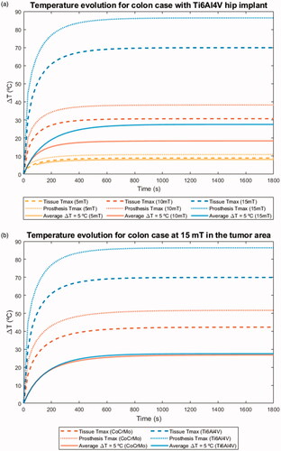
Table 4. Main parameters from the curves featured in Figure 6 (threshold ΔT = 5 °C, maximum temperature in tissue, and maximum temperature in prosthesis).

	Time (s)
	Figure 6(a) (Ti6Al4V)			Figure 6(b) (15 mT)
Parameter	5 mT	10 mT	15 mT	Ti6Al4V	CoCrMo
Threshold ΔT = 5 °C	540	690	930	930	1020
Maximum temperature in tissue	540	690	870	870	990
Maximum temperature in prosthesis	570	720	900	900	1020

The reported time values are those so that the derivative of the temperature vs time curves is less than 0.001 s.

These curves also reveal how quickly a particular set of conditions may cause harm to tissues adjacent to the prostheses. In principle, such damage may occur in as much and as long as they surpass the recommended thresholds by the ICNIRP. This is particularly important for high intensity values, since thermal thresholds may be exceeded from the beginning of the treatment and maximum temperatures may be reached before the therapeutic temperature is attained at the tumor site.

Only data at the highest field intensity is shown here to provide a better insight in the safety issues. Nevertheless, the obtained data for the remaining indications under lower field intensities are freely available in the supplementary information [66]. In those cases, there is a variable time period before the thermal thresholds start to be surpassed.

4. Conclusions

We have presented a methodology aimed to revise and improve the current exclusion criteria applied to implant-bearing patients in magnetic hyperthermia treatments, increasing their chances of inclusion and hence the access to a better quality of life. The studied prostheses heat up in all the tested field conditions, which include a range of relevant H·f values, in some cases higher than those used in clinical trials and thus providing a good case for risk estimation. We have established that the secondary field produced by eddy currents at the surface of the implants creates a maximum distortion of about 1–2 cm thick just around the hip joint, which in practical terms means that the effective field keeps unperturbed for most of the radiated regions.

We have seen that thermal equilibrium at both the prosthesis and tissues is reached at a time point ranging from 540 s to 1020s, depending on the combination of field conditions and choice of prosthesis material. Consequently, the effective therapy time at the desired temperature may be actually the half of the overall one, and thus this transient period toward thermal equilibrium should be carefully appraised during treatment planning. Besides the methodology for predicting prosthesis heating, we propose a quick screening method based on calculated SAR and temperature data plotted in a log-log graph, which in turn is divided in four quadrants, each representing different levels of severity of tissue damage. Of particular note is that the proposed methodology allowed to discern the basic underlying mechanisms to the temperature elevation (field-tissue interaction, heat exchange from field-implant interaction) over the treated region. Whereas for some conditions – for example, prostate cancer at 15 mT – the therapy is rendered unsafe given the high temperatures reached at bone tissues, for others the therapy may be safe – for example, colorectal cancer at 5 mT for any type of implant biomaterial. In any case, the benefit/risk ratio of undergoing the procedure under some given conditions must be carefully appraised by the clinical staff. Our simulations have also established differences and similarities between the biomaterials from which the implants were made.

Very likely, the current stringent admission criteria that completely exclude implant-bearing patients is due to the lack of systematic preclinical studies, both costly and complex to be carried out in humans. Nevertheless, systematic in silico treatment planning, backed by an adequate methodology, can help in recovering for this minimally invasive therapy those otherwise excluded patients who could benefit greatly from it.

Disclosure statement

No potential conflict of interest was reported by the author(s).

Data availability statement

The whole dataset obtained during the course of this study is publicly available for download. The files are uploaded in the Zenodo repository under the title ‘Dataset from “In silico assessment of collateral eddy current heating in biocompatible implants subjected to magnetic hyperthermia treatments”.’ The structure of the files is also explained [66].

Additional information

Funding

This work has been supported by the NoCanTher project, which has received funding from the European Union’s Horizon 2020 research and innovation programme under grant agreement No [685795]. The authors acknowledge support from the COST Association through the COST actions ‘RADIOMAG’ [TD1402] and ‘MyWAVE’ [CA17115]. D.O. and I.R.R. acknowledge financial support from the Community of Madrid under Contract No. [PEJD-2017-PRE/IND-3663], from the Error! Hyperlink reference not valid. through the Ramón y Cajal grant [RYC2018-025253-I] and Research Networks [RED2018-102626-Hiroshima], as well as the Ministry of Economy and Competitiveness through the grants [MAT2017-85617-R] and the ‘Severo Ochoa’ Program for Centers of Excellence in R&D [SEV-2016-0686]. We gratefully acknowledge the support of NVIDIA Corporation through the GPU Grant Program with the donation of the Quadro P6000 GPU used for this research. D. O. acknowledges support from the Programme for the Promotion and Encouragement of Research and Transfer activities at the University of Cadiz.

References

- Johannsen M, Gneveckow U, Eckelt L, et al. Clinical hyperthermia of prostate cancer using magnetic nanoparticles: presentation of a new interstitial technique. Int J Hyperthermia. 2005;21:637–647.
- Johannsen M, Gneveckow U, Taymoorian K, et al. Morbidity and quality of life during thermotherapy using magnetic nanoparticles in locally recurrent prostate cancer: results of a prospective phase I trial. Int J Hyperthermia. 2007;23:315–323.
- Ortega D, Pankhurst QA. Magnetic hyperthermia. In: O'Brien P, editor. Nanoscience: volume 1: nanostructures through chemistry. Cambridge (UK): The Royal Society of Chemistry; 2013. p. 60–88.
- Kirui DK, Celia C, Molinaro R, et al. Mild hyperthermia enhances transport of liposomal gemcitabine and improves in vivo therapeutic response. Adv Healthc Mater. 2015;4:1092–1103.
- Niiyama E, Uto K, Lee CM, et al. Hyperthermia nanofiber platform synergized by sustained release of paclitaxel to improve antitumor efficiency. Adv Healthcare Mater. 2019;8:1900102.
- Starsich FHL, Sotiriou GA, Wurnig MC, et al. Silica-coated nonstoichiometric nano Zn-ferrites for magnetic resonance imaging and hyperthermia treatment. Adv Healthc Mater. 2016;5:2698–2706.
- Paulides MM, Stauffer PR, Neufeld E, et al. Simulation techniques in hyperthermia treatment planning. Int J Hyperthermia. 2013;29:346–357.
- Lagendijk JJW. Hyperthermia treatment planning. Phys Med Biol. 2000;45:R61–R76.
- Gellermann J, Wust P, Stalling D, et al. Clinical evaluation and verification of the hyperthermia treatment planning system hyperplan. Int J Radiat Oncol Biol Phys. 2000;47:1145–1156.
- Seebass M, Beck R, Gellermann J, et al. Electromagnetic phased arrays for regional hyperthermia: optimal frequency and antenna arrangement. Int J Hyperthermia. 2001;17:321–336.
- Sreenivasa G, Gellermann J, Rau B, et al. Clinical use of the hyperthermia treatment planning system HyperPlan to predict effectiveness and toxicity. Int J Radiat Oncol Biol Phys. 2003;55:407–419.
- Maier-Hauff K, Ulrich F, Nestler D, et al. Efficacy and safety of intratumoral thermotherapy using magnetic iron-oxide nanoparticles combined with external beam radiotherapy on patients with recurrent glioblastoma multiforme. J Neurooncol. 2011;103:317–324.
- Maier-Hauff K, Rothe R, Scholz R, et al. Intracranial thermotherapy using magnetic nanoparticles combined with external beam radiotherapy: results of a feasibility study on patients with glioblastoma multiforme. J Neurooncol. 2007;81:53–60.
- Rakow A, Schoon J, Dienelt A, et al. Influence of particulate and dissociated metal-on-metal hip endoprosthesis wear on mesenchymal stromal cells in vivo and in vitro. Biomaterials. 2016;98:31–40.
- Pearson MJ, Williams RL, Floyd H, et al. The effects of cobalt-chromium-molybdenum wear debris in vitro on serum cytokine profiles and T cell repertoire. Biomaterials. 2015;67:232–239.
- Andrä W, Nowak H. Magnetism in medicine: a handbook. Weinheim (Germany): John Wiley & Sons; 2007.
- Maradit-Kremers H, Crowson CS, Larson D, et al. Prevalence of total hip (THA) and total knee (TKA) arthroplasty in the United States. Proceedings of the American Academy of Orthopaedic Surgeons 2014 Annual Meeting; 2014; New Orleans, LA.
- Neufeld E, Kühn S, Szekely G, et al. Measurement, simulation and uncertainty assessment of implant heating during MRI. Phys Med Biol. 2009;54:4151–4169.
- Murbach M, Zastrow E, Neufeld E, et al. Heating and safety concerns of the radio-frequency field in MRI. Curr Radiol Rep. 2015;3:45.
- Cabot E, Lloyd T, Christ A, et al. Evaluation of the RF heating of a generic deep brain stimulator exposed in 1.5 T magnetic resonance scanners. Bioelectromagnetics. 2013;34:104–113.
- Córcoles J, Zastrow E, Kuster N. Convex optimization of MRI exposure for mitigation of RF-heating from active medical implants. Phys Med Biol. 2015;60:7293–7308.
- Zilberti L, Bottauscio O, Chiampi M, et al. Collateral thermal effect of MRI-LINAC gradient coils on metallic hip prostheses. IEEE Trans Magn. 2014;50:1–4.
- Zilberti L, Bottauscio O, Chiampi M, et al. Numerical prediction of temperature elevation induced around metallic hip prostheses by traditional, split, and uniplanar gradient coils. Magn Reson Med. 2015;74:272–279.
- Arduino A, Bottauscio O, Chiampi M, et al. Douglas–Gunn method applied to dosimetric assessment in magnetic resonance imaging. IEEE Trans Magn. 2017;53:1–4.
- Brühl R, Ihlenfeld A, Ittermann B. Gradient heating of bulk metallic implants can be a safety concern in MRI. Magn Reson Med. 2017;77:1739–1740.
- Atkinson WJ, Brezovich IA, Chakraborty DP. Usable frequencies in hyperthermia with thermal seeds. IEEE Trans Biomed Eng. 1984;31:70–75.
- Haider SA, Cetas TC, Wait JR, et al. Power absorption in ferromagnetic implants from radiofrequency magnetic fields and the problem of optimization. IEEE Trans Microwave Theory Techn. 1991;39:1817–1827.
- Kobayashi T, Kida Y, Ohta M, et al. [Magnetic induction hyperthermia for brain tumor using ferromagnetic implant with low curie temperature. Effect on intracutaneously implanted brain tumor]. Neurol Med Chir. 1986;26:116–121.
- DRKS-ID: DRKS00005476, MF 1001: Open-label, randomized, controlled study to determine the efficacy and safety of NanoTherm® monotherapy and NanoTherm® in combination with radiotherapy versus radiotherapy alone in recurrent/progressive glioblastoma, German Clinical Trials Register, 2013.
- Ahlbom A, Bergqvist U, Bernhardt JH, et al. Guidelines for limiting exposure to time-varying electric, magnetic, and electromagnetic fields (up to 300 GHz). Health Phys. 1998;74:494–521.
- Adibzadeh F, Paulides MM, van Rhoon GC. SAR thresholds for electromagnetic exposure using functional thermal dose limits. Int J Hyperthermia. 2018;34:1248–1254.
- Stauffer PR, Cetas TC, Fletcher AM, et al. Observations on the use of ferromagnetic implants for inducing hyperthermia. IEEE Trans Biomed Eng. 1984;31:76–90.
- ICNIRP (International Commission on Non-Ionizing Radiation Protection). Guidelines for limiting exposure to electromagnetic fields (100 kHz to 300 GHz). Health Phys. 2020;118:483–524.
- ICNIRP (International Commission on Non-Ionizing Radiation Protection). ICNIRP statement on the “Guidelines for limiting exposure to time-varying electric, magnetic, and electromagnetic fields (up to 300 GHz). Health Phys. 2009;97:257–258.
- Lin J, Saunders R, Schulmeister K, et al. ICNIRP Guidelines for limiting exposure to time-varying electric and magnetic fields (1 Hz to 100 kHz). Health Phys. 2010;99:818–836.
- Stigliano RV, Shubitidze F, Petryk JD, et al. Mitigation of eddy current heating during magnetic nanoparticle hyperthermia therapy. Int J Hyperthermia. 2016;32:735–748.
- Neufeld E, Gosselin M, Sczcerba D, et al. Sim4Life: a medical image data based multiphysics simulation platform for computational life sciences. Proceedings of the VPH 2012 Congress (VPH 2012); 2012; London, UK.
- Bottauscio O, Chiampi M, Hand J, et al. A GPU computational code for eddy-current problems in voxel-based anatomy. IEEE Trans Magn. 2015;51:1–4.
- Bottauscio O, Chiampi M, Zilberti L. Massively parallelized boundary element simulation of voxel-based human models exposed to MRI fields. IEEE Trans Magn. 2014;50:1029–1032.
- Bottauscio O, Cassarà AM, Hand JW, et al. Assessment of computational tools for MRI RF dosimetry by comparison with measurements on a laboratory phantom. Phys Med Biol. 2015;60:5655–5680.
- Pennes HH. Analysis of tissue and arterial blood temperatures in the resting human forearm. J Appl Physiol. 1948;1:93–122.
- Laakso I, Hirata A. Dominant factors affecting temperature rise in simulations of human thermoregulation during RF exposure. Phys Med Biol. 2011;56:7449–7471.
- Gosselin MC, Neufeld E, Moser H, et al. Development of a new generation of high-resolution anatomical models for medical device evaluation: the Virtual Population 3.0. Phys Med Biol. 2014;59:5287–5303.
- Christ A, Kainz W, Hahn EG, et al. The Virtual Family-development of surface-based anatomical models of two adults and two children for dosimetric simulations. Phys Med Biol. 2010;55:N23–N38.
- Hasgall P, di Gennaro F, Baumgartner C, et al. IT’IS Database for thermal and electromagnetic parameters of biological tissues.
- Gouasmi S. 2014 [accessed 2019 Feb 8]. Dental implant. https://grabcad.com/library/dental-implant-1
- Wang R. 2016 [accessed 2019 Feb 8]. Hip implant. https://grabcad.com/library/hip-implant-1
- Blender 2.79. 2017 [accessed 2020 Apr 22]. https://www.blender.org/
- Périgo EA, Hemery G, Sandre O, et al. Fundamentals and advances in magnetic hyperthermia. Appl Phys Rev. 2015;2:041302.
- Blanco-Andujar C, Teran FJ, Ortega D. Chapter 8 - Current outlook and perspectives on nanoparticle-mediated magnetic hyperthermia. In: Mahmoudi M, Laurent S, editors. Iron oxide nanoparticles for biomedical applications. Amsterdam (Netherlands): Elsevier; 2018. p. 197–245.
- Gneveckow U, Jordan A, Scholz R, et al. Description and characterization of the novel hyperthermia- and thermoablation-system MFH 300F for clinical magnetic fluid hyperthermia. Med Phys. 2004;31:1444–1451.
- EU Horizon 2020 project ‘NoCanTher: Nanomedicine upscaling for early clinical phases of multimodal cancer therapy’. European Commission; 2016.
- Arduino A, Bottauscio O, Brühl R, et al. In silico evaluation of the thermal stress induced by MRI switched gradient fields in patients with metallic hip implant. Phys Med Biol. 2019;64:245006.
- Head WC, Bauk DJ, Emerson RH Jr. Titanium as the material of choice for cementless femoral components in total hip arthroplasty. Clin Orthop Relat Res. 1995;(311):85–90.
- http://www.matweb.com/search/datasheet.aspx?MatGUID=a0655d261898456b958e5f825ae85390 [accessed 2021 Apr 6].
- Tanaka Y, Saito H, Tsutsumi Y, et al. Active hydroxyl groups on surface oxide film of titanium, 316L stainless steel, and cobalt-chromium-molybdenum alloy and its effect on the immobilization of poly(ethylene glycol). Mater Trans. 2008;49:805–811.
- Starčuková J, Starčuk Z, Hubálková H, et al. Magnetic susceptibility and electrical conductivity of metallic dental materials and their impact on MR imaging artifacts. Dent Mater. 2008;24:715–723.
- MACBETH (Measuring Attractiveness by a Categorical Based Evaluation Technique), Wiley Encyclopedia of Operations Research and Management Science; 2011.
- Hirata A, Shirai K, Fujiwara OJPIER. On averaging mass of SAR correlating with temperature elevation due to a dipole antenna. PIER. 2008;84:221–237.
- Hirata A, Laakso I, Oizumi T, et al. The relationship between specific absorption rate and temperature elevation in anatomically based human body models for plane wave exposure from 30 MHz to 6 GHz. Phys Med Biol. 2013;58:903–921.
- Dossel O, Bohnert J. Safety considerations for magnetic fields of 10 mT to 100 mT amplitude in the frequency range of 10 kHz to 100 kHz for magnetic particle imaging. Biomed Eng. 2013;58:611–621.
- Gleich B, Weizenecker J. Tomographic imaging using the nonlinear response of magnetic particles. Nature. 2005;435:1214–1217.
- Graeser M, Thieben F, Szwargulski P, et al. Human-sized magnetic particle imaging for brain applications. Nat Commun. 2019;10:1936.
- IEEE Standard for Safety Levels with Respect to Human Exposure to Radio Frequency Electromagnetic Fields, 3 kHz to 300 GHz, IEEE Std C95.1-2005 (Revision of IEEE Std C95.1-1991). 2006. p. 1–238.
- IEEE Standard for Safety Levels with Respect to Human Exposure to Electric, Magnetic, and Electromagnetic Fields, 0 Hz to 300 GHz, IEEE Std C95.1-2019 (Revision of IEEE Std C95.1-2005/Incorporates IEEE Std C95.1-2019/Cor 1-2019). 2019. p. 1–312.
- Rubia-Rodríguez I, Zilberti L, Arduino A, et al. Dataset from "In silico assessment of collateral eddy current heating in biocompatible implants subjected to magnetic hyperthermia treatments. (Version 3.1.2). Int J Hyperthermia. 2020.
- Panagopoulos DJ, Johansson O, Carlo GL. Evaluation of specific absorption rate as a dosimetric quantity for electromagnetic fields bioeffects. PLOS One. 2013;8:e62663.
- Marsh K, Goetghebeur M, Thokala P, et al. Multi-criteria decision analysis to support healthcare decisions. Cham (Switzerland): Springer; 2017.
- Peng Q, Juzeniene A, Chen J, et al. Lasers in medicine. Rep Prog Phys. 2008;71:056701.
- Bana CA, Costa E, Vansnick J-C. Applications of the MACBETH approach in the framework of an additive aggregation model. J Multi-Crit Decis Anal. 1997;6:107–114.
- Angelis A, Montibeller G, Hochhauser D, et al. Multiple criteria decision analysis in the context of health technology assessment: a simulation exercise on metastatic colorectal cancer with multiple stakeholders in the English setting. BMC Med Inform Decis Mak. 2017;17:149.
- Broekhuizen H, Groothuis-Oudshoorn CGM, Hauber AB, et al. Estimating the value of medical treatments to patients using probabilistic multi criteria decision analysis. BMC Med Inform Decis Mak. 2015;15:102.
- Yarmolenko PS, Moon EJ, Landon C, et al. Thresholds for thermal damage to normal tissues: an update. Int J Hyperthermia. 2011;27:320–343.
- Goldstein LS, Dewhirst MW, Repacholi M, et al. Summary, conclusions and recommendations: adverse temperature levels in the human body. Int J Hyperthermia. 2003;19:373–384.
- Dewhirst MW, Viglianti BL, Lora-Michiels M, et al. Basic principles of thermal dosimetry and thermal thresholds for tissue damage from hyperthermia. Int J Hyperthermia. 2003;19:267–294.
- Johannsen M, Gneveckow U, Thiesen B, et al. Thermotherapy of prostate cancer using magnetic nanoparticles: feasibility, imaging, and three-dimensional temperature distribution. Eur Urol. 2007;52:1653–1662.
- Pennes HH. Analysis of tissue and arterial blood temperatures in the resting human forearm. 1948. J Appl Physiol (1985). 1998;85:5–34.