Validation of a coupled electromagnetic and thermal model for estimating temperatures during magnetic nanoparticle hyperthermia

Abstract

Purpose

Alternating magnetic field (AMF) tissue interaction models are generally not validated. Our aim was to develop and validate a coupled electromagnetic and thermal model for estimating temperatures in large organs during magnetic nanoparticle hyperthermia (MNH).

Materials and methods

Coupled finite element electromagnetic and thermal model validation was performed by comparing the results to experimental data obtained from temperatures measured in homogeneous agar gel phantoms exposed to an AMF at fixed frequency (155 ± 10 kHz). The validated model was applied to a three-dimensional (3D) rabbit liver built from computed tomography (CT) images to investigate the contribution of nanoparticle heating and nonspecific eddy current heating as a function of AMF amplitude.

Results

Computed temperatures from the model were in excellent agreement with temperatures calculated using the analytical method (error < 1%) and temperatures measured in phantoms (maximum absolute error <2% at each probe location). The 3D rabbit liver model for a fixed concentration of 5 mg Fe/cm³ of tumor revealed a maximum temperature ∼44 °C in tumor and ∼40 °C in liver at AMF amplitude of ∼12 kA/m (peak).

Conclusion

A validated coupled electromagnetic and thermal model was developed to estimate temperatures due to eddy current heating in homogeneous tissue phantoms. The validated model was successfully used to analyze temperature distribution in complex rabbit liver tumor geometry during MNH. In future, model validation should be extended to heterogeneous tissue phantoms, and include heat sink effects from major blood vessels.

Keywords:

• Hyperthermia
• magnetic nanoparticles
• eddy currents
• electromagnetic modeling
• bioheat transfer
• gel phantom
• verification and validation

Introduction

Magnetic nanoparticle hyperthermia (MNH) is approved by the European Medicines Agency to treat recurrent glioblastoma in combination with RT in 2010 [1] and received an investigational device exemption (IDE) approval from US FDA in 2018 to conduct prostate cancer clinical trials [2]. MNH is the selective heating of cancerous tissue using magnetic nanoparticles which generate heat when exposed to an alternating magnetic field (AMF) [3,4]. The potential offered by MNH to produce effective localized heating compared to other hyperthermia modalities makes it attractive in clinical scenarios requiring precise control of thermal dose [5–7]. Three-dimensional temperature monitoring technologies such as magnetic resonance thermal imaging (MRTI) is not compatible with MNH. Current MNH treatment planning and monitoring systems use image based bioheat transfer modeling and invasive single or multiple point thermometry respectively [5–7]. However, validated electromagnetic and bioheat transfer model-based treatment planning, and quality control is not a reality for MNH as for radiofrequency, microwave and interstitial hyperthermia approaches [8–14].

Treatment planning frameworks for MNH are mostly based on bioheat transfer models with magnetic nanoparticle deposits as heating source and ignore the AMF tissue-interactions generating tissue heating due to induced eddy currents [1,5,15–19]. Various approaches such as pulsed AMF [20,21], relative motion [22] and AMF amplitude modulation [23] have been proposed to reduce nonspecific eddy current heating and improve temperature distribution in tumors. Implementing the above-mentioned complex algorithms in a clinical setting requires a fully coupled electromagnetic and thermal modeling framework accounting for AMF-tissue interactions along with the bioheat transfer component.

Such fully coupled electromagnetic and thermal models should integrate both “absorption” based eddy-current heating due to AMF-tissue interaction, ‘loss (hysteresis)’ based magnetic nanoparticle heating and thermoregulatory responses such as vasodilation or collapse in capillaries, and heat sink effects of larger nearby blood vessels [24–28]. Rigorous validation of the fully coupled electromagnetic and thermal treatment planning models are limited as only few clinical [15,17] and preclinical [29,30] AMF systems are calibrated and fully characterized.

Nonspecific eddy current heating intensifies when large volumes of tissue are exposed to a strong AMF to treat deep-seated tumors in pancreas, liver, prostate and rectum [26,31]. Power deposited by eddy currents, per unit volume in tissues, historically reported as ‘specific absorption rate’ (SAR), increases with AMF amplitude and frequency, and radius of the eddy current path [32–35]. Thus, this square-dependence of power deposited by eddy currents on the magnetic field amplitude limits the use of high AMF amplitudes to increase thermal dose deposited in a clinical setting [15–17,31,36]. Additionally, eddy current heating depends on tissue material properties, geometry, tissue interfaces and radius of the eddy current path [30–35]. However, the complex geometry and heterogeneity of tissue properties makes it difficult to monitor eddy currents and eddy current heating during MNH. The safety limits due to eddy current heating vary with anatomical locations. For example, AMF exposure of the pelvic region during MNH treatment was limited due to the eddy current heating observed in skin folds [31]. Superficial cooling methods such as cooling pads used to remove heat from the skin surface are not effective beyond 2 cm due to the conductive limits [30–32].

Heat generated by anatomically targeted magnetic nanoparticles is critical for achieving required thermal in the tumors. Magnetic nanoparticle heating is often reported as specific loss power (SLP) [3,32]. Magnetic nanoparticle SLP exhibits a nonlinear power dependence on applied AMF amplitude and generally, a linear dependence on frequency. Significant progress has been achieved in improving nanoparticle SLPs [37–41].

In addition to heat generation sources, computational bioheat-transfer modeling considers the heat losses due to conduction, convection and perfusion changes in the tumor and the surrounding tissue. Power deposition in tissues, and consequent heating can initiate a thermoregulatory response in the patient that results in perfusion changes affecting temperatures that are realized in both target and off-target regions. Multiple bioheat transfer models exist to account for the thermoregulatory response [42–46].

Tissue equivalent gel phantoms and computational modeling are previously used to understand eddy current heating [47,48] but were not extensively validated with experimental data. Stigliano et al. [48] conducted a partial validation of their model by comparing their simulated temperature with measured temperatures in an agar gel phantom only at a single time point. Additionally, the effect of input parameter uncertainties on the simulated eddy current heating and temperatures was not considered. The primary means to assess accuracy and reliability of any computational model is by verification and validation [49]. Assessment of the accuracy of a solution to a computational model with known solutions (often analytical) is known as verification. Validation, on the other hand, is the assessment of the accuracy of a computational solution by comparison with experimental data [49]. It is therefore important to verify and validate a computational model before using it for devising treatment strategies or understanding of complex phenomena. There is an immediate need to develop a validated coupled electromagnetic and thermal modeling framework for reliable treatment planning systems with emphasis on AMF-tissue interactions. In this study we developed a coupled thermal and electromagnetic model for estimating temperature due to eddy current heating for a homogeneous tissue phantom. The model was verified and validated using analytical methods and experimental data. Uncertainty analysis was carried out to estimate the uncertainties in the computed temperature distributions and to determine the parameters that have the most influence on the computed temperature distributions. Previously reported magnetic nanoparticle heating (SLP) and the thermal regulatory response models [21,23,29,39] were used in conjunction with the validated model to study the contribution of nanoparticle heating and nonspecific eddy current heating as function of AMF amplitude in a three-dimensional rabbit liver built from computed tomography images.

Materials and methods

Coupled electromagnetic and heat transfer model

Electromagnetic and heat transfer analysis was carried out with commercially available multi-physics finite element solver (COMSOL Multiphysics, Natick, MA), on a cylindrical geometry shown in Figure 1. The dimensions and tissue properties were chosen to approximate a human organ such as the liver (Table 1) [50]. The computational model has three concentric cylinders and is built to represent the exposed tissue inside a magnetic coil with superficial cooling system, which is representative of the experimental setup described previously [30]. The innermost cylinder represents the tissue equivalent gel phantom, outermost cylinder represents the region of active uniform applied magnetic field generated by an AMF coil [30], and the middle cylinder represents the water jacket, a superficial cooling system used in magnetic hyperthermia [30].

Figure 1. (a) Schematic of the computational model considered in the study computational model consists of three concentric cylindrical domains with the innermost domain being the gel phantom, the second layer being the water jacket and the outermost being the magnetic coil. (b) Sample mesh plot of the computational domains. (c) Three locations along the radius where temperatures were compared.

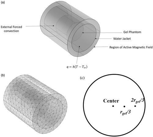
Table 1. Mean parameter values and their uncertainties considered in the simulations.

Parameter	Mean value	Uncertainty
Magnetic field amplitude (kA/m)	6.96	±10% [36]
Frequency (kHz)	160	±10% [36]
Electrical Conductivity (S/m)	0.3325 [38]	±10% [38]
Density (kg/m^3)	960	±5%
Specific heat capacity (J/kg-K)	3900 [41]	±10% [41]
Thermal conductivity (W/m-K)	0.566 [42]	±5% [42]
Diameter of gel (m)	0.103	±0.5 mm
Height of gel (m)	0.093	±0.5 mm
Position along radius of gel (cm)	0	±5 mm
Position along axis of gel (cm)	7.0	±5 mm
Probe location (cm)	0.05, 1.85, 3.45	±3 mm
Water jacket temperature (°C)	20	±0.5 °C
Ambient temperature (°C)	20	±1 °C

Electromagnetic and heat transfer simulations were simultaneously carried out by coupling Maxwell’s equations and transient heat conduction equation. The effect of alternating magnetic field on the cylindrical gel phantom with electrical conductivity, σ, can be described by Maxwell’s equations: (1) $$\nabla \times H=\mathrm{J}$$(1) (2) $$B=\mathrm{ }\nabla \mathrm{ }\times A$$(2) (3) $$E=\mathrm{ }-j\omega A$$(3) (4) $$J=\text{ σE}+\text{jωD},$$(4)

where J is the current density, $\omega \mathrm{ }$ is the angular frequency, H is the magnetic field intensity, A is the magnetic vector potential, E is the electric field intensity, B is the magnetic flux density and D is electric flux density. Heat transfer in the gel phantom due the heat generated by induced eddy currents can be described by, (5) $$\rho c_p\frac{\partial T}{\partial t}=k{\nabla }^{2}T+Q_{\mathit{eddy}}$$(5) where ρ is the density, c_p is the specific heat, T is the temperature, k is the thermal conductivity and Q_eddy is the heat produced due to eddy currents. The boundary conditions for the electromagnetic modeling, given by a uniform AMF field of amplitude H and frequency f, was imposed on the surface of the coil. For heat transfer modeling, the surfaces of the water jacket were subjected to an external forced convection boundary condition with plate averaged heat transfer coefficient, given by (6) $$q_o=h_{\mathit{conv}}\mathrm{ }(T-T_{\mathit{ext}})$$(6) (7) $$h_{\mathit{conv}}=h_{\mathit{water}}(L,U,T_{\mathit{ext}})$$(7) where L is the length of the water jacket, U is the water flow velocity and T_ext is the water temperature. The open faces of the water jacket were modeled by free convection boundary condition given by, (8) $$q=h_{\mathit{free}}(T-T_{\mathrm{\infty }})$$(8) where T_∞ is the ambient temperature and h_free is the free convection heat transfer coefficient. The thermal and electrical properties used in the simulations are summarized in Table 1.

Equations (1)–(8) were coupled and simultaneously solved using finite element analysis. Sensitivity of the solution to grid size and time step size were carried out to ensure choice of mesh size and time step had negligible effect on the computed temperature.

Verification with analytical model

The analytical expression for the volumetric power absorbed by a cylindrical tissue of radius r exposed to an alternating magnetic field of constant amplitude H and frequency f is given by, (9) $$P_{\mathit{tissue}}={\pi }^2\frac{{\mu }_0^2\sigma }{2}{f}^2{H}^2{r}^2$$(9) where µ_o is the permeability of free space and σ is the electrical conductivity [30,32,51,52]. This equation is valid only for constant field amplitude H, uniform tissue electrical conductivity σ, and when$\sqrt{f\sigma {\mu }_o}{r}_{\mathit{max}}\ll 1$ [29,51,52]. The computational model was verified with the analytical model by comparing and plotting the computed temperatures at three locations along the radius (Figure 1(c)).

Validation with experimental model

Alternating magnetic field system

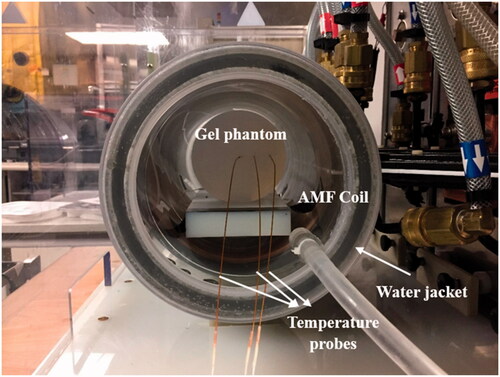
A uniform AMF was generated in the region of interest using a 20 cm diameter modified Maxwell coil (AMF Life Systems, Auburn Hills, MI) shown in Figure 2, connected to a 120 kW induction heating power supply (PPECO, Watsonville, CA) [36]. A commercially available two-dimensional magnetic field probe (AMF Life Systems, Auburn Hills, MI) was used to measure the field inside the coil [30]. The field was uniform (<10% variation) in a cylindrical region of 10 cm in length and 16 cm in diameter for the AMF amplitudes up to ∼22 kA/m at 155 ± 10 kHz. A polyacrylic water jacket (Figure 2) was inserted into the coil to minimize the heat transfer between the gel and the coil. It was connected to a recirculating chiller (ThermoFlex, Thermo Fisher Scientific, Newington, NH) which was maintained at 20 °C [30].

Figure 2. Experimental setup for the gel phantom experiments. Agar gel phantoms were inserted in the center of a 20-cm horizontal modified Maxwell coil inside a water jacket with temperature controlled at 20 °C. Temperatures were measured at the center of the gel, r_gel/3, and 2r_gel/3 distance along the radius of the gel, where r is the gel radius.

Gel phantom model

Cylindrical gel phantoms (Figure 2) were prepared by heating a solution of 1% agarose (Type I-A, low EEO, Sigma Aldrich, St. Louis, MO, Lot #SLBC0292V), with sodium chloride, crystal (J. T. Baker, Lot K17586) in 750 ml of distilled deionized water. The solution was heated using a heating plate and a magnetic stirrer until all the agar were dissolved in the solution. The solution was then allowed to solidify and cool to room temperature for more than 12 h to ensure uniform temperature inside the gel. The dimensions of the gel were then measured using a measuring scale. The electrical conductivity of the gel was calculated using [53], (10) $$\sigma \left[\frac{S}{m}\right]=215\times \frac{\mathit{Grams}\mathrm{ }of\mathrm{ }\mathit{sodium}\mathrm{ }\mathit{chloride}}{\mathit{solution}\mathrm{ }\mathit{volume}\mathrm{ }\left(mL\right)}+0.0529$$(10)

The gel phantom could equilibrate to room temperature for more than 12 h before inserting it into the coil. The gel was then inserted into the coil and exposed to a constant alternating magnetic field of amplitude 13.94 kA/m (peak to peak) and at fixed frequency 160 kHz (observed) for 15 min. Temperatures were measured radially at three locations (r = 0, r_gel/3, 2r_gel/3) where r is the radial distance from gel center, at the center of the gel (H_gel/2) using optical fiber temperature probes (accuracy: ±0.3 °C, resolution: 0.1 °C and response time <750 ms; FISO Technologies, Ltd., Quebec, Canada). These measurements were then used to compare with the computed temperatures for validation of the computational model.

Uncertainty analysis

The root-sum-square (RSS) model [54–56] was used to calculate temperature uncertainties in our computational model. The temperature at any time can be represented as a function of all input model parameters: (11) $$T=g(p_1,p_2,p_3,\dots \dots ,p_n)$$(11)

here $p_1,p_2,p_3,\dots \dots ,p_n$ are the individual parameters.

Assuming the value of each parameter is independently associated with an uncertainty δ, the uncertainty in the temperature distribution can be calculated as, (12) $$T\pm \delta T=\mathrm{ }g(p_1\pm \delta p_1,p_2\pm \delta p_2,p_3\pm \delta p_3,\dots \dots ,p_n\pm \delta p_n)$$(12)

The uncertainty in the temperature distribution is then given by [54–58], (13) $$\pm \delta T=\sum _{i=1}^n\frac{\partial g}{\partial p_i}\delta p_i$$(13)

The partial derivatives can be computed by: (14) $$\frac{\partial g}{\partial p_i}\delta p_i\cong \mathrm{ }\frac{T_i-T_0}{\Delta p_i}\delta p_i={[T_i-T_0]}_{\Delta p_i=\delta p_i}\equiv \Delta T_i$$(14)

The overall uncertainty can then be calculated as [54–58]: (15) $$\delta T=\sqrt{\sum _{i=1}^n{\left(\frac{\partial g}{\partial p_i}\delta p_i\right)}^2}$$(15)

In our current model, the temperature T generated in the gel due to eddy current heating depends on the gel dimensions, such as diameter (D_gel), height (H_gel), thermal properties such as density (ρ), thermal conductivity (k) and specific heat capacity (c_p), electrical conductivity (σ), applied magnetic field conditions like magnetic field intensity (H), frequency (f), the gel position inside the coil determined with respect to the coil center given by radial distance of the center of the gel from coil center (x_pos) and along the axis of the coil (y_pos), and the location of the probe. The mean values of the parameters based on recorded data and/or applied conditions are shown in Table 1. The relative permittivity for the gel was chosen as 1. The ambient temperature was measured using a standard room thermometer and the water jacket temperature was measured using a fiber-optic temperature probe [59]. The uncertainty in the temperatures at the three probe locations (±3 mm) was calculated by iteration with varying uncertainties of individual parameters while holding all others fixed, using parameters and nominal uncertainty values listed in Table 1. A 5% difference between of the computed temperatures and the measured temperature was considered acceptable for the model validation.

Application to three-dimensional (3D) models of rabbit liver obtained from computed tomography (CT) images

CT images of rabbit liver

X-ray CT images of a randomly selected rabbit VX2 liver tumor model from an ongoing liver cancer study was used to build a 3D liver model for simulations. The ongoing liver cancer study used adult white New Zealand rabbits. All animals were housed in an Association for Assessment and Accreditation of Laboratory Animal Care (AAALAC) - accredited facility in compliance with the guide for the care and use of laboratory animals. All procedures were approved by the Johns Hopkins Institutional Animal Care and Use Committee (IACUC). At specific time points, each animal was selected for VX2 tumor implantation in the liver and subsequently underwent CT imaging to monitor tumor growth before experimental intervention.

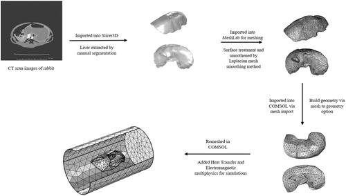
The CT images of rabbit were imported into an open-source software, 3DSlicer [60], for visualization and medical image computing. Automatic segmentation does not yield a desirable result due to the overlapping gray level values of the soft tissue organs. 3DSlicer was used to manually segment and differentiate the liver from the other organs using the gray level value and apply smoothing algorithms to the region of interest. Manual segmentation was performed to differentiate the liver from other organs by choosing the lower and higher threshold gray level value. Segmented files were converted into a 3D surface geometry CAD (.stl) format. The meshing of the liver CAD geometry was performed using a Laplacian mesh smoothing method in MeshLab® [61]. Several iterations of mesh smoothing were carried out to ensure a well smoothened geometry. Surface treatment and defeaturing were performed to smooth sharp edges and artifacts obtained in reconstructed geometries to ensure compliance of the meshed geometry (.stl file) with finite element simulation software. The workflow of building 3D models from CT scan images is shown in Figure 3.

Figure 3. Workflow for building 3 D models of rabbit liver from CT scan images: CT scan images of rabbit liver were first imported into Slicer3D and the liver was extracted by manual segmentation. The file was then imported into MeshLab for meshing and smoothing of sharp edges to allow for import into finite element software for simulations. File was then imported into COMSOL via mesh import option and converted into geometry. The geometry is then remeshed in COMSOL and multi-physics is added for simulations.

Computational liver model

Coupled electromagnetic and heat transfer simulations were then carried out on the CT image-based liver model and the geometry considered is shown in Figure 4. The computational geometry mainly consists of three domains: (1) the extracted liver domain, (2) spherical tumor inside the liver and (3) rabbit torso/tissue approximated as a cylinder. The spherical tumor was arbitrarily introduced close to the liver domain center. Heat transfer in the tissues were modeled using the Pennes bioheat equation [62], given by (16) $${\rho }_n{c}_n\frac{\partial T_n}{\partial t}=k_n{\nabla }^2{T}_n+{\rho }_b{c}_b{\omega }_{b,n}\mathrm{ }\left({\mathrm{ }T}_b-T_n\mathrm{ }\right)+Q_{m,n}+Q_{\mathit{eddy}}+Q_{\mathrm{p}}$$(16) where subscripts n and b represent tissue (liver, n = 1; tumor, n = 2; tissue, n = 3) and blood; respectively. ρ_n, c_n, k_n, T_n and Q_m,n denote the density, specific heat, thermal conductivity, local temperature, metabolic heat generation rate, for either tumor or healthy tissue and t is the heating time, $Q_{\mathit{eddy}}$ is the heating rate per unit volume due to eddy currents and Q_p is the heating rate per unit volume of tumor due to nanoparticles. ρ_b, c_b, ω_b,n and T_b denote density, specific heat, perfusion rate and temperature, of blood, respectively. Constant perfusion was considered in the current study for ease of computation and to gain preliminary insights into the temperature distributions. The thermal and electrical properties of the tissues considered in the model were given in Table 2 and Table 3. The nanoparticle heating rate was modeled using the previously reported specific loss power (SLP) values of magnetic iron oxide nanoparticles [39] and the continuous polynomial approximation given by Soetaert et al. [63]. It was assumed that the nanoparticles were only present in the tumor. The concentration of nanoparticles was chosen as 5 mg Fe/cc of tumor, to be consistent with previous studies [21,23,64,65].

Figure 4. Schematic of the computational model used for simulations. (a) Isometric projection of the geometry showing the liver, tumor and rabbit tissue/torso. Thermal and magnetic field boundary conditions are shown. (b) Sample mesh for the computational model shown in (a).

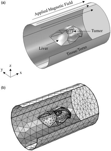
Table 2. Thermal properties of tissues considered in the present study.

	Density, ρ (kg/m^3)	Specific heat, c (J/kg K)	Thermal conductivity, k (W/m K)	Blood perfusion rate, ω (1/s)	Metabolic heat generation rate, Qm (W/m^3)
Liver	1079 [50]	3540 [50]	0.52 [50]	0.018 [51]	14,414 [52]
Tumor	1079 [50]	3540 [50]	0.52 [50]	0.018 [51]	72,070 [53]
Tissue/torso	1090 [50]	3421 [50]	0.49 [50]	0.0027 [53]	684.2 [53]
Blood^a	1060 [54]	3770 [54]	N/A	N/A	N/A

^aTemperature of blood (T_b) was fixed at 37 °C [54].

N/A: not applicable.

Table 3. Electrical properties of tissue used in the simulations.

	Electrical conductivity, σ (S/m)	Relative permittivity
Liver	0.0954 [50]	6090 [50]
Tumor	0.0954 [50]	6090 [50]
Tissue/Torso	0.373 [50]	7110 [50]

Thermal boundary conditions considered for this model are free convection boundary condition at all the outside boundaries of the tissue/torso domain (Equation (17)) and the continuity of temperature and heat flux at the domain interfaces. (17) $$q=h_{\mathit{free}}(T-T_{\mathrm{\infty }})$$(17) where T_∞ is the ambient temperature (20 °C) and h_free is the free convection heat transfer coefficient (10 W/m²-K). For the electromagnetic boundary conditions, magnetic fields of 4−20 kA/m (peak) at a fixed frequency of 150 kHz are applied on the outer boundaries of the tissue/torso layer. Simulations were carried out for a treatment duration of 20 min at constant amplitude and the resulting temperature distributions were computed.

Results

Verification and validation of computational model-based treatment planning framework to mitigate eddy current heating is required to improve the quality control and assurance of MNH in the clinic. In this study, we present a rigorously verified and validated coupled thermal and electromagnetic model for predicting temperatures produced due to eddy current heating.

Verification with analytical model

The temperature distribution in the computational cylindrical phantom after 15 min exposure to a constant alternating magnetic field of 13.94 kA/m at a fixed frequency of 160 kHz is shown in Figure 5(a). It can be observed that temperatures increase away from the phantom center, with the lowest temperatures at the center and highest at the periphery. Higher temperatures simulated generated in regions away from the phantom center is consistent with that predicted by the analytical solution (Equation (9)), where the heat generated is proportional to the square of the distance from the center of the field.

Figure 5. (a) Isothermal contours showing the temperature distributions achieved inside the phantom after 15 min of exposure to an alternating magnetic of 13.97 kA/m at a fixed frequency of 160 kHz, (b) verification of computational model with analytical solution. Comparison of computed temperatures with the coupled electromagnetic and heat transfer model with temperatures calculated using the analytical expression for power absorption at center of gel shows excellent agreement.

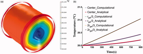
The constraint for using the analytical expression (Equation (9)), $\sqrt{f\sigma {\mu }_o}{r}_{\mathit{max}}$ ≪ 1, was satisfied for the modeled scenario. The computed temperatures at three locations in the phantom, center, r_gel/3 and 2r_gel/3 were compared to the corresponding temperatures calculated using the analytical expression and plotted in Figure 5(b). Excellent agreement (error < 1%) was seen between the computed temperatures and the calculated temperatures using the analytical expression, thus verifying the computational model.

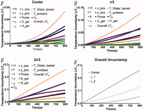
Uncertainty analysis and validation with experimental data

Potential parameters capable of significantly influencing the simulation outcome were identified for estimation of uncertainties. Uncertainty analysis was carried out for the identified simulation input parameters reported in Table 1. The uncertainty in computed temperatures due to individual parameter uncertainties and the overall uncertainty is shown in Figure 6. Temperature uncertainty was plotted at three locations: center of the phantom, r_gel/3 distance from the phantom center, and 2r_gel/3 distance from phantom center.

Figure 6. Overall uncertainty in temperatures as a function of time measured at the center, r_gel/3, and 2r_gel/3, due to uncertainty in individual parameters identified in Table 1. The variation in overall uncertainty of temperature with time was plotted for each probe location. Computed temperatures are most sensitive to the uncertainties in applied field (H), frequency (f), probe placement (Probe), specific heat capacity (C_p), electrical conductivity (σ) and gel density (ρ). Note r_1 and r_2 represent rgel/3, and 2rgel/3, respectively.

The computed temperatures were compared with the experimental measurements for validation of the computational model. The computed and measured temperatures fall within the range of ±5% with all the corresponding uncertainties at all the three probe locations, leading to an acceptable validation of the developed computational model. However, we tested the model more rigorously by determining the parameter values that fit the computed temperatures at the center to the measured values (difference of <5%) and using these parameter values we compared the computed and measured temperatures at the other two locations (r_gel/3 and 2r_gel/3). The parameter values were the mean values reported in Table 1 for all the parameters, except for H, Cp and ρ. The uncertainty in probe placement was still shown as this was independent of the gel properties and coil properties. The computed and measured temperatures were then plotted for each of the locations along with probe placement uncertainties and shown in Figure S1. Excellent agreement was observed between the computed and measured values with the maximum absolute error <2% at each of the probe location.

3D models of rabbit liver

The verified and validated coupled thermal and electromagnetic model was then implemented on a 3D liver model generated from CT scan images as shown in Figure 4. Nanoparticle heating was considered to estimate and understand the temperatures achieved in the liver and tumor, because of nanoparticles and eddy current heating. Simulations were performed for a range of constant magnetic field amplitudes of 4−20 kA/m (peak) at a fixed frequency of 150 kHz for a duration of 20 min, with and without nanoparticle heating. The nanoparticle heating was modeled using previously reported SLP values for magnetic iron oxide nanoparticles [39,63,66]. The temperature distributions obtained in the liver after 100 and 1200s of exposure to a constant applied magnetic field of 20 kA/m with no nanoparticle heating are shown in Figure 7(a). Temperature gradients can be observed in the liver, with the temperatures closer to the liver center being lower and increasing radially away, resulting in the maximum temperatures achieved on the liver edges. After 20 min of exposure, considerable heating occurs with a maximum of ∼40 °C observed at the liver edges. At higher fields, hyperthermic temperatures (41−43 °C) can be obtained in the liver due to eddy current heating.

Figure 7. (a) Temperature distribution in the liver after 20 min of exposure to an AMF amplitude of 20 kA/m (peak) at a fixed frequency of 150 kHz. Elevated temperatures can be observed at the edges of the liver with temperature of ∼40 °C at the end of 20 min of exposure. (b) Maximum temperatures achieved in the tumor, liver and surrounding superficial tissue during 20 min of AMF exposure at 12 kA/m and 50 kHz. Maximum temperatures achieved in the liver and tumor after 20 min of exposure to an AMF amplitude of 4 to 20 kA/m (peak) at a fixed frequency of 150 kHz with (c) no nanoparticle heating and (d) with nanoparticle heating.

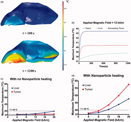
The maximum temperatures achieved in the liver and tumor is shown in Figure 7(b–d). In case of the model without nanoparticles, the observed temperatures in the liver rise with increase in applied magnetic field due to increased eddy current generation, while no significant increase in tumor temperatures is observed. When nanoparticle heating is included, higher tumor temperature was observed compared to liver. Additionally, the maximum temperature in the liver with nanoparticles is higher (at 16 kA/m, 43.8 °C compared to 38.9 °C with no nanoparticles), due to heat transfer from the nanoparticle heat sources.

Discussion

MNH offers significant advantages for controlled deposition of heat in a targeted tissue region [1,6]. Volume dependent off-target induced eddy current heating is an important factor for patient safety. Eddy current heating increases at higher applied field amplitudes and frequency limiting the efficacy of MNH especially when large tissue volumes are exposed to AMF in the clinic [30,33–35]. Effective methods to manage eddy current heating [20–22,30] are critical to treating deep-seated tumors of liver, pancreas and prostate. The complexity in tissue geometries and heterogeneity in tissue properties makes it challenging to monitor eddy currents and eddy current heating in humans in real-time during MNH.

A primary challenge in validating a computational model with experimental data arises from uncertainties of the simulation input parameters. Neglecting the uncertainties associated with the measured data yields incorrect results of either invalidating a correct model or validating an incorrect model [54–58,67].

Uncertainty analysis of the developed coupled electromagnetic and thermal model shows that the temperature uncertainty was most sensitive to the parameters that affect heat generation followed by parameters that affect heat transfer. The parameters that influence heat generation are applied magnetic field amplitude H, frequency f, probe location (radial distance from phantom center) and electrical conductivity σ. The parameters that influence heat transfer are density ρ, specific heat capacity C_p, thermal conductivity k, and temperatures of water jacket and ambient. As predicted uncertainties in the parameters that influence heat generation had the greatest influence on computed temperatures. The rate of heat generation, given by Equation (9), is proportional to the square of the product Hf. Hence, variability in either of them had a strong effect on the computed temperatures. Of the other parameters, the next sensitive parameter was probe location (radial distance from center). This was also expected as the heat generation term is directly proportional to the square of the distance (r) from the center. The variability in electrical conductivity σ, had the next significant effect on the computed temperatures. Of the parameters that influence heat transfer, the variability in specific heat C_p and density ρ, had the most effect on the computed temperatures. When the overall uncertainty was compared for each of the three locations, the uncertainty increased significantly as we moved away from the phantom center.

The tumor location with respect to the eddy current heating zones could be an important factor to influencing the delivered thermal dose in the target region. For superficial tumors eddy current heating can add to the deposited thermal dose in the targeted region for circumferential coil designs (Figure 7(b,c)). This is consistent with several preclinical studies reporting a 2–3 °C increase in the animal’s skin surface temperature due to eddy current heating [68–72]. The developed model successfully simulates the eddy current heating in large organs such as liver and highlights the importance of considering heating due to eddy currents when optimizing magnetic nanoparticle hyperthermia for clinical studies. Use of a limited number of temperature probes is a limitation in the current study. Use of infrared (IR) thermal camera, and multi-point (up to eight probes) gallium arsenide (GaAs) fiberoptic temperature bundle (FISO Technologies, Ltd., Quebec, Canada.) would allow for a significantly greater number of data points, to enhance temperature measurements in more complex (heterogeneous) in vivo tissues and organs. Current validated model can be used to develop effective strategies to minimizing the off-target eddy current heating and improve safety of MNH.

Validation of coupled electromagnetic and bioheat transfer model is critical to improve the quality control and assurance of MNH in the clinic. This study represents the first step to developing such validated model. Future studies will focus on verification and validation of the nanoparticle heating and thermal regulatory response components of the treatment planning system. Future efforts should also include heterogeneous phantoms [73–75] and in vivo models accounting for tissue properties, tumor geometry, nanoparticle distribution, blood flow associated with small vessels and capillaries, location of large blood vessel [76,77] and AMF tissue interaction at tissue interfaces. These, however, will require organ/tissue specific imaging and model parameters, give the substantial differences in the various anatomical locations that present with cancer. Heterogenous phantom can be based on a soaked porous structure with closed loop flow [78] to simulate the blood flow associated with small vessels and capillaries. Limited temperature data is a major limitation of the current study. Detailed temperature mapping is critical for the validation of future heterogeneous and in vivo models. A combination of multi-point GaAs fiberoptic temperature bundle, infrared camera, and/or thermochromic films can facilitate a detailed temperature mapping. Heterogeneous and in vivo validation models should focus on replicating clinically relevant scenarios such as low magnetic nanoparticle concentration in target region, amplitude modulation to reduce nonspecific eddy current heating [21], and spatial localization target thermal dose using gradient fields to avoid off-target thermal damage [79].

Future FEA models would include hybrid bioheat transfer, (a) conjugate heat transfer between large blood vessels to account for the heat sink effect and (b) volume average approach based on Pennes bioheat equation for the blood flow associated with small vessels and capillaries. Successful development of an MNH treatment planning system will need a development of methods to measure patient specific temperature dependent tissue properties such as blood perfusion and electrical conductivity.

Disclosure statement

R.I. and E.L. are inventors of nanoparticle patents. All patents are assigned to either the Johns Hopkins University or Aduro Biosciences, Inc. R.I. consults for Imagion Biosystems and Magnetic Insight and is a member of the Scientific Advisory Board of Imagion Biosystems. All other authors report no conflicts of interest. Additional financial support (A.A.) was provided by School of Science, Engineering, and Technology, the Pennsylvania State University – Harrisburg. The contents of this article is solely the responsibility of the authors and do not necessarily represent the official view of the Pennsylvania State University, Johns Hopkins University, JKTGF, NIH and other funding agencies.

Additional information

Funding

R.I. and E.L. received partial funding from the National Cancer Institute (5R01 CA194574-02). R.I received partial funding from the Jayne Koskinas and Ted Giovanis Foundation for Health and Policy (JKTGF). R.I. and A.A. received partial funding from the National Cancer Institute (5R01 CA247290).

References

- Maier-Hauff K, Ulrich F, Nestler D, et al. Efficacy and safety of intratumoral thermotherapy using magnetic iron-oxide nanoparticles combined with external beam radiotherapy on patients with recurrent glioblastoma multiforme. J Neurooncol. 2011;103(2):317–324.
- MagForce AG. The nanomedicine company. U.S. FDA IDE approval to start prostate cancer study. Shareholder letter; 2019. Available from: https://www.magforce.com/fileadmin/user_upload/MagForce_AG_Shareholder_Letter_June_20_2019.pdf.
- Dennis CL, Ivkov R. Physics of heat generation using magnetic nanoparticles for hyperthermia. Int J Hyperthermia. 2013;29(8):715–729.
- Chandrasekharan P, Tay ZW, Hensley D, et al. Using magnetic particle imaging systems to localize and guide magnetic hyperthermia treatment: tracers, hardware, and future medical applications. Theranostics. 2020;10(7):2965–2981.
- LeBrun A, Zhu L. Magnetic nanoparticle hyperthermia in cancer treatment: History, mechanism, imaging‐assisted protocol design, and challenges. In: Shrivastava D, editor. Theory and Applications of Heat Transfer in Humans. Hoboken, NJ: Wiley; 2018. p. 631–667.
- Ivkov R. Magnetic nanoparticle hyperthermia: a new frontier in biology and medicine? Int J Hyperthermia. 2013;29(8):703–705.
- Mahmoudi K, Bouras A, Bozec D, et al. Magnetic hyperthermia therapy for the treatment of glioblastoma: a review of the therapy’s history, efficacy and application in humans. Int J Hyperth. 2018;34(8):1316–1328.
- Trefná HD, Crezee H, Schmidt M, et al. Quality assurance guidelines for superficial hyperthermia clinical trials: I. Clinical requirements. Int J Hyperthermia. 2017;33(4):471–482.
- Dobšíček Trefná H, Crezee J, Schmidt M, et al. Quality assurance guidelines for superficial hyperthermia clinical trials : II. Technical requirements for heating devices. Strahlenther Onkol. 2017;193(5):351–366.
- Dobšíček Trefná H, Schmidt M, van Rhoon GC, et al. Quality assurance guidelines for interstitial hyperthermia. Int J Hyperthermia. 2019;36(1):276–293.
- Mulder HT, Curto S, Paulides MM, et al. Systematic quality assurance of the BSD2000-3D MR-compatible hyperthermia applicator performance using MR temperature imaging. Int J Hyperthermia. 2018;35(1):305–313.
- Kok HP, Kotte AN, Crezee J. Planning, optimisation and evaluation of hyperthermia treatments. Int J Hyperthermia. 2017;33(6):593–607.
- Kok HP, Korshuize-van Straten L, Bakker A, et al. Online adaptive hyperthermia treatment planning during locoregional heating to suppress treatment-limiting hot spots. Int J Radiat Oncol Biol Phys. 2017;99(4):1039–1047.
- Schooneveldt G, Löke DR, Zweije R, et al. Experimental validation of a thermophysical fluid model for use in a hyperthermia treatment planning system. Int J Heat Mass Transf. 2020;152:119495.
- Gneveckow U, Jordan A, Scholz R, et al. Description and characterization of the novel hyperthermia- and thermoablation-system MFH 300F for clinical magnetic fluid hyperthermia. Med Phys. 2004;31(6):1444–1451.
- Johannsen M, Thiesen B, Wust P, et al. Magnetic nanoparticle hyperthermia for prostate cancer. Int J Hyperthermia. 2010;26(8):790–795.
- Johannsen M, Gneveckow U, Thiesen B, et al. Thermotherapy of prostate cancer using magnetic nanoparticles: feasibility, imaging, and three-dimensional temperature distribution. Eur Urol. 2007;52(6):1653–1662.
- LeBrun A, Manuchehrabadi N, Attaluri A, et al. MicroCT image-generated tumour geometry and SAR distribution for tumour temperature elevation simulations in magnetic nanoparticle hyperthermia. Int J Hyperthermia. 2013;29(8):730–738.
- LeBrun A, Joglekar T, Bieberich C, et al. Identification of infusion strategy for achieving repeatable nanoparticle distribution and quantification of thermal dosage using micro-CT Hounsfield unit in magnetic nanoparticle hyperthermia. Int J Hyperthermia. 2016;32(2):132–143.
- Ivkov R, DeNardo SJ, Daum W, et al. Application of high amplitude alternating magnetic fields for heat induction of nanoparticles localized in cancer. Clin Cancer Res. 2005;11(19):7093s–70103.
- Attaluri A, Kandala SK, Zhou H, et al. Magnetic nanoparticle hyperthermia for treating locally advanced unresectable and borderline resectable pancreatic cancers: the role of tumor size and eddy-current heating. Int J Hyperthermia. 2020;37(3):108–119.
- Stigliano RV, Shubitidze F, Petryk JD, et al. Mitigation of eddy current heating during magnetic nanoparticle hyperthermia therapy. Int J Hyperthermia. 2016;32(7):735–748.
- Kandala SK, Liapi E, Whitcomb LL, et al. Temperature-controlled power modulation compensates for heterogeneous nanoparticle distributions: a computational optimization analysis for magnetic hyperthermia. Int J Hyperthermia. 2019;36(1):115–129.
- Miaskowski A, Subramanian M. Numerical model for magnetic fluid hyperthermia in a realistic breast phantom: calorimetric calibration and treatment planning. IJMS. 2019;20(18):4644. Jan
- Bellizzi G, Bucci OM. On the optimal choice of the exposure conditions and the nanoparticle features in magnetic nanoparticle hyperthermia. Int J Hyperthermia. 2010;26(4):389–403.
- Bellizzi G, Bucci OM, Chirico G. Numerical assessment of a criterion for the optimal choice of the operative conditions in magnetic nanoparticle hyperthermia on a realistic model of the human head. Int J Hyperthermia. 2016;32(6):688–703.
- Adhikary K, Banerjee M. A thermofluid analysis of the magnetic nanoparticles enhanced heating effects in tissues embedded with large blood vessel during magnetic fluid hyperthermia. J Nanopart Res. 2016;2016:1–18.
- Tang Y, Jin T, Flesch RC. Numerical temperature analysis of magnetic hyperthermia considering nanoparticle clustering and blood vessels. IEEE Trans Magn. 2017;53(10):1–6.
- Attaluri A, Nusbaum C, Wabler M, et al. Calibration of a quasi-adiabatic magneto-thermal calorimeter used to characterize magnetic nanoparticle heating. J Nanotechnol Eng Med. 2013;4(1):011006.
- Attaluri A, Jackowski J, Sharma A, et al. Design and construction of a Maxwell-type induction coil for magnetic nanoparticle hyperthermia. Int J Hyperthermia. 2020;37(1):1–4.
- Johannsen M, Gneveckow U, Taymoorian K, et al. Morbidity and quality of life during thermotherapy using magnetic nanoparticles in locally recurrent prostate cancer: results of a prospective phase I trial. Int J Hyperthermia. 2007;23(3):315–323.
- Kumar A, Attaluri A, Mallipudi R, et al. Method to reduce non-specific tissue heating of small animals in solenoid coils. Int J Hyperthermia. 2013;29(2):106–120.
- Atkinson WJ, Brezovich IA, Chakraborty DP. Usable frequencies in hyperthermia with thermal seeds. IEEE Trans Biomed Eng. 1984;31(1):70–75. BME
- Jordan A, Wust P, Fähling H, et al. Inductive heating of ferrimagnetic particles and magnetic fluids: physical evaluation of their potential for hyperthermia. Int J Hyperthermia. 1993;9(1):51–68.
- Young JH, Wang MT, Brezovich I. Frequency/depth-penetration considerations in hyperthermia by magnetically induced currents. Electron Lett. 1980;16(10):358–359.
- Wust P, Gneveckow U, Johannsen M, et al. Magnetic nanoparticles for interstitial thermotherapy-feasibility, tolerance and achieved temperatures. Int J Hyperthermia. 2006;22(8):673–685.
- Lee JH, Jang JT, Choi JS, et al. Exchange-coupled magnetic nanoparticles for efficient heat induction. Nat Nanotechnol. 2011;6(7):418–422.
- Dennis CL, Jackson AJ, Borchers JA, et al. The influence of collective behavior on the magnetic and heating properties of iron oxide nanoparticles. J Appl Phys. 2008;103(7):07A319.
- Bordelon DE, Cornejo C, Grüttner C, et al. Magnetic nanoparticle heating efficiency reveals magneto-structural differences when characterized with wide ranging and high amplitude alternating magnetic fields. J Appl Phys. 2011;109(12):124904.
- Woodard LE, Dennis CL, Borchers JA, et al. Nanoparticle architecture preserves magnetic properties during coating to enable robust multi-modal functionality. Sci Rep. 2018;8(1):1–3.
- He S, Zhang H, Liu Y, et al. Maximizing specific loss power for magnetic hyperthermia by hard–soft mixed ferrites. Small. 2018;14(29):1800135.
- Shrivastava D, Vaughan JT. A generic bioheat transfer thermal model for a perfused tissue. J Biomechanical Eng. 2009;131(7):074506.
- Shrivastava D. Alternate thermal models to predict in vivo temperatures. In: Shrivastava D, editor. Theory and applications of heat transfer in humans. Hoboken, NJ: Wiley; 2018. p. 15–23.
- Tompkins DT, Vanderby R, Klein SA, et al. Temperature-dependent versus constant-rate blood perfusion modelling in ferromagnetic thermoseed hyperthermia: results with a model of the human prostate. Int J Hyperthermia. 1994;10(4):517–536.
- Kok HP, Gellermann J, van den Berg CA, et al. Thermal modelling using discrete vasculature for thermal therapy: A review. Int J Hyperthermia. 2013;29(4):336–345.
- Nakayama A, Kuwahara F. A general bioheat transfer model based on the theory of porous media. Int J Heat Mass Transf. 2008;51(11-12):3190–3199.
- Di Barba P, Dughiero F, Sieni E, et al. Coupled field synthesis in magnetic fluid hyperthermia. IEEE Trans Magn. 2011;47(5):914–917.
- Stigliano RV, Shubitidze F, Petryk AA, et al. Magnetic nanoparticle hyperthermia: Predictive model for temperature distribution. Proc Soc Photo Opt Instrum Eng. 2013. 8584:858410.
- Oberkampf WL, Trucano TG, Hirsch C. Verification, validation, and predictive capability in computational engineering and physics. Appl Mech Rev. 2004;57(5):345–384.
- Wolf DC. Evaluation of the size, shape, and consistency of the liver. Clin Methods Hist Phys Lab Exam. 1990;62(6):478–481.
- Stauffer PR, Cetas TC, Jones RC. Magnetic induction heating of ferromagnetic implants for inducing localized hyperthermia in deep-seated tumors. IEEE Trans Biomed Eng. 1984;31(2):235–251. BME
- Brezovich I. Low frequency hyperthermia: capacitive and ferromagnetic thermoseed methods. Med Phys Monogr. 1988;16:82–111.
- Bennett D. NaCl doping and the conductivity of agar phantoms. Mater Sci Eng C. 2011;31(2):494–498.
- Standard for verification and validation in computational fluid dynamics and heat transfer – ASME V V 20; 2009.
- Assessing credibility of computational modeling through verification and validation: application to medical devices ASME V V 40; 2018.
- Rabin Y. A general model for the propagation of uncertainty in measurements into heat transfer simulations and its application to cryosurgery. Cryobiology. 2003;46(2):109–120.
- NIST/SEMATECH e-Handbook of Statistical Methods. Available from: http://www.itl.nist.gov/div898/handbook/
- Kline SJ. The purposes of uncertainty analysis. J Fluids Eng. 1985;107(2):153–160.
- FISO FOT-M Temperature sensor [Internet]. [cited 2017 Feb 8]. Available from: https://www.fiso.com/admin/useruploads/files/fot-m.pdf.
- 3D Slicer [Internet]. [cited 2017. Feb 8]. Available from: https://www.slicer.org/.
- MeshLab [Internet]. [cited 2017. Feb 8]. Available from: http://www.meshlab.net/.
- Pennes HH. Analysis of tissue and arterial blood temperatures in the resting human forearm. J Appl Physiol. 1948;1(2):93–122.
- Soetaert F, Dupré L, Ivkov R, et al. Computational evaluation of amplitude modulation for enhanced magnetic nanoparticle hyperthermia. Biomed Tech. 2015;60(5):491–504.
- Attaluri A, Kandala SK, Wabler M, et al. Magnetic nanoparticle hyperthermia enhances radiation therapy: a study in mouse models of human prostate cancer. Int J Hyperthermia. 2015;31(4):359–374.
- Attaluri A, Seshadri M, Mirpour S, et al. Image-guided thermal therapy with a dual-contrast magnetic nanoparticle formulation: A feasibility study. Int J Hyperthermia. 2016;32(5):543–557.
- Hedayati M, Attaluri A, Bordelon D, et al. New iron-oxide particles for magnetic nanoparticle hyperthermia: an in-vitro and in-vivo pilot study. Proc SPIE 2013;8584:858404.
- Coleman HW, Stern F. Uncertainties and CFD code validation. J Fluids Eng Asme. 1997;119(4):795–803.
- Rodrigues HF, Mello FM, Branquinho LC, Zufelato N, et al. Real-time infrared thermography detection of magnetic nanoparticle hyperthermia in a murine model under a non-uniform field configuration. Int J Hyperthermia. 2013;29(8):752–767.
- Kolosnjaj-Tabi J, Di Corato R, Lartigue L, et al. Heat-generating iron oxide nanocubes: subtle “destructurators” of the tumoral microenvironment. ACS Nano. 2014;8(5):4268–4283.
- Di Corato R, Béalle G, Kolosnjaj-Tabi J, et al. Combining magnetic hyperthermia and photodynamic therapy for tumor ablation with photoresponsive magnetic liposomes. ACS Nano. 2015;9(3):2904–2916.
- Espinosa A, Di Corato R, Kolosnjaj-Tabi J, et al. Duality of iron oxide nanoparticles in cancer therapy: amplification of heating efficiency by magnetic hyperthermia and photothermal bimodal treatment. ACS Nano. 2016;10(2):2436–2446.
- Rodrigues HF, Capistrano G, Mello FM, et al. Precise determination of the heat delivery during in vivo magnetic nanoparticle hyperthermia with infrared thermography. Phys Med Biol. 2017;62(10):4062–4082.
- Yuan Y, Wyatt C, Maccarini P, et al. A heterogeneous human tissue mimicking phantom for RF heating and MRI thermal monitoring verification. Phys Med Biol. 2012;57(7):2021–2037.
- Mobashsher AT, Abbosh AM. Artificial human phantoms: human proxy in testing microwave apparatuses that have electromagnetic interaction with the human body. IEEE Microwave. 2015;16(6):42–62.
- Kaczmarek K, Mrówczyński R, Hornowski T, et al. The effect of tissue-mimicking phantom compressibility on magnetic hyperthermia. Nanomaterials. 2019;9(5):803.
- Yue K, Zheng S, Luo Y, et al. Determination of the 3D temperature distribution during ferromagnetic hyperthermia under the influence of blood flow. J Therm Biol. 2011;36(8):498–506.
- Javidi M, Heydari M, Attar MM, et al. Cylindrical agar gel with fluid flow subjected to an alternating magnetic field during hyperthermia. Int J Hyperthermia. 2015;31(1):33–39.
- Tofighi MR, Attaluri A. Closed-loop pulse-width modulation microwave heating with infrared temperature control for perfusion measurement. IEEE Trans Instrum Meas. 2021;70:1–7.
- Tay ZW, Chandrasekharan P, Chiu-Lam A, et al. Magnetic particle imaging-guided heating in vivo using gradient fields for arbitrary localization of magnetic hyperthermia therapy. ACS Nano. 2018;12(4):3699–3713.