Modeling accumulated degree-days for the invasive aquatic plant Oxycaryum cubense in the southeastern United States

Abstract

Cuban bulrush (Oxycaryum cubense [Poepp. & Kunth] Lye) is an invasive floating aquatic plant that causes negative ecological and economic impacts in the southeastern United States. Temperatures in the United States have increased over recent decades which can result in geographic expansion of invasive plants in North America. Accumulated degree-days (ADD) were utilized to develop predictive models (state and regional models) for Cuban bulrush growth from harvested biomass collected over one year in Mississippi, Louisiana, and Florida. Peak emergent biomass occurred from early to mid-fall (September-October) with growth continuing into winter. Accumulated degree days needed for Cuban bulrush to reach peak emergent biomass ranged from 6,469 (Mississippi), 7111 (regional), 7,643 (Florida), and 7,903 (Louisiana). Calendar days needed for Cuban bulrush to reach peak emergent biomass ranged from 292 (Mississippi) to 334 (Florida). Base temperature thresholds for Cuban bulrush were −6 C, −3 C, −3 C, and −2 C for Mississippi, Louisiana, regional, and Florida models respectively. The models suggest Cuban bulrush has a tolerance to lower air temperatures that could allow for survival in moderate winter conditions. Overall, model predictability was less accurate for populations further south (Florida) due to warmer winter temperatures, year-round growth, and difficulty defining when peak emergent biomass occurred. Results from this study indicate that Cuban bulrush growth is greater in warmer temperatures, though low base temperature thresholds suggest this species may be capable of expanding its invaded range to cooler climates beyond the southeastern United States.

Keywords:

• Cuban bulrush
• heat units
• predictive modeling
• polycephalous
• monocephalous
• peak biomass

Introduction

Cuban bulrush [Oxycaryum cubense (Poepp. & Kunth) Lye] is an epiphytic perennial invasive plant that exploits other aquatic plants or structures for habitat and does not directly rely on sediment roots or belowground biomass for most of its life cycle (Bryson et al. 2008). It is native to the tropical Americas and is found throughout the southeastern United States where both types of terminal inflorescences are found, multiple head (polycephalous) (Oxycaryum cubense forma cubense) and single head (monocephalous) (Oxycaryum cubense forma paraguayense) (Bryson et al. 2008; Bryson and Carter 2008). Cuban bulrush is stoloniferous which allows for vegetative reproduction; however, it also produces single seeded achenes which are buoyant and allow for water dispersal (Bryson and Carter 2008; Grippo et al. 2014; Watson and Madsen 2014). Cuban bulrush relies on plants like Eichhornia crassipes (Mart.) Solms and Salvinia molesta D.S. Mitch as a seed germination and structurally supporting substrate (McFarland et al. 2004; Bryson et al. 2008).

The current invaded distribution includes parts of Africa, Mexico, and throughout the southeastern United States (Carter 2005; Bryson et al. 2008; Bryson and Carter 2008; Grippo et al. 2014; Sartain et al. 2014). The first record of Cuban bulrush in the United States was in 1878 on the eastern side of Mobile Bay in Alabama (SERNEC 2022 McNeal UNA00001491; Mohr UNA00001486); however, it is also thought to have arrived in Florida around the same time (Chapman 1889). Cuban bulrush was likely introduced by migratory birds or ship ballast from the tropical Americas (Bryson and Carter 2008; Grippo et al. 2014). Historic records of the 1878 population found in Alabama described both inflorescence forms, with both forms originating from the tropical Americas (SERNEC 2022 McNeal UNA00001491; Mohr UNA00001486). The plant is commonly found along the water’s edge, or floating freely within freshwater ditches, ponds, lakes, rivers, swamps, and marshes (Bryson et al. 2008, Grippo et al. 2014). With the ability to rapidly colonize new waterways, Cuban bulrush infestations impact multi-use lakes, reservoirs, flowing waters that provide drinking water, hydro-electric power, fish, outdoor recreational activities, and navigation for commercial and military vessels (Watson and Madsen 2014, Turnage and Shoemaker 2017). Being an emergent plant, temperature is an important driver in seasonal life history and expansion of its current range (Kriticos and Brunel 2016; Vose et al. 2017).

Temperatures in the United States have increased 1.8 °C from 1895 to 2016 with most of that increase (0.7 °C) occurring from 1981 to 2016 (Kriticos and Brunel 2016; Vose et al. 2017). Several climate models predict a 3 to 9 °C increase in the United States over the next century (Finch et al. 2021). Additionally, increases in temperature results in increased plant productivity due to increased rates of physiological processes (Riis et al. 2012), which suggests the ranges of several invasive species may expand in response to increases in temperature (Kriticos and Brunel 2016; Vose et al. 2017; IPCC 2022). Accumulated degree-day models have been used previously to predict plant growth for aquatic plants throughout an annual cycle (Spencer et al. 2000); or to determine influences of variables, such as air temperature, on critical portions of a plant’s life cycle (peak biomass production) (Squires et al. 2024). Predicting these life cycle events can help resource managers more accurately monitor spread or to plan management efforts to target vulnerable points in a plant’s life cycle.

Accumulated degree-days are a measure of heat units used to predict the occurrence of transition points (e.g. sprouting, flowering, peak height, peak biomass) in a plant’s life cycle (Snyder 1985; Hayhoe and Dwyer 1990; Arazi et al. 1993; Yang et al. 1994; Forcella and Banken 1996; McMaster and Wilhelm 1997; Roltsch et al. 1999; Snyder et al. 1999; Spencer et al. 2000). Accumulated heat is also known as physiological time (Zalom et al. 1983). Physiological time is measured in degree days, where one degree day is equal to one degree above the lower developmental threshold over a 24 h period. Researchers often want to know how many degree-days are needed for crops to sprout, or how many degree-days are needed before flowering is observed, or maximum plant height is observed (Snyder 1985; Hayhoe and Dwyer 1990; Arazi et al. 1993; Sanderson et al. 1994; Yang et al. 1994; Forcella and Banken 1996; McMaster and Wilhelm 1997; Roltsch et al. 1999; Snyder et al. 1999; Spencer et al. 2000).

Accumulated degree days are calculated as the sum of daily degree-days across a developmental stage (Zalom et al. 1983). Degree-days can be calculated from temperature measurements compounded over flexible temporal scales (e.g. hourly, daily, weekly), but are often recorded as the mean daily temperature (Snyder et al. 1999), though some species have temperature thresholds below or above which no growth is seen. Thus, in many cases threshold temperatures are unknown and need to be calculated (Snyder et al. 1999). The lower developmental threshold, or the base threshold, is the temperature below which physiological processes or plant development stops (Zalom et al. 1983; UC IPM 2016). Since ADD is based on temperature accumulation (rather than time), the predictive capability is somewhat immune to changes in geographic location within a region when upper and lower threshold temperatures are incorporated (Snyder 1985; Snyder et al. 1999; Spencer et al. 2000). Consequently, accumulated degree days needed to complete a life stage at one location should be comparable to ADD estimated at another location even though calendar days needed to achieve the life stage may be different at each site (Snyder 1985; Snyder et al. 1999; Spencer et al. 2000).

The current literature describing environmental influences to Cuban bulrush growth is sparse. To date there is only one study that has documented the phenology and life history of Cuban bulrush in the United States (Clarke et al. 2023); and a second that used ADD modeling to predict base threshold temperatures and heat units needed for Cuban bulrush to achieve peak biomass in a growing season (Squires et al. 2024). However, these previous studies were spatially limited in their sampling area. It is generally assumed that Cuban bulrush cannot tolerate freezing temperatures (Grippo et al. 2014); yet, data from Mississippi populations suggest Cuban bulrush may be metabolically active at air temperatures as low as −4 °C (Squires et al. 2024). Given the limited spatial extent of previous studies, additional research is needed to determine the utility of ADD modeling at greater (regional) spatial scales. By including more populations from the southeastern United States, the predictive ability of ADD models may improve by capturing more spatial and temporal variability in regional temperature and Cuban bulrush growth. Therefore, the objectives of this study were to 1) develop and compare state specific ADD models predicting peak biomass of Cuban bulrush harvested from Mississippi, Florida, and Louisiana, and 2) develop a regional ADD model incorporating greater spatial and temporal data. Modeling data can inform natural resource managers as to the potential range expansion of invasive species and be used in the development of early detection and rapid response programs.

Methods

Biomass data collection

A field study was conducted using established Cuban bulrush populations at Lake Columbus near Columbus, Mississippi (33°32′ 2.76″ N, 88°29′ 27.60″ W), Lake Martin near Lafayette, Louisiana (30°13′ 23.2572″ N, 91°54′22.284″ W), and Orange Lake between Gainesville and Ocala, Florida (29°27′ 32.39″ N, 82°10′23.40″ W). Plots in Mississippi were established by placing PVC posts into the lakebed at the corners of each plot. Each corner post was then geotagged in case of damage from flooding or other natural events. Louisiana and Florida plots were marked with plot centers that were also geotagged; samples were collected within 10 m of plot centers. Sites were located in secluded areas that were less likely to be affected by disturbance or management. From October 2021 to September 2022, Cuban bulrush was harvested monthly from two 0.04 Ha plots in each site. At each site, twelve random samples were collected using a 0.1 m² (33 cm x 33 cm) quadrat to quantify Cuban bulrush biomass. All plants were cut within the perimeter of the quadrat, placed in labeled 3.79-L plastic storage bags, and stored in a cooler. Samples from all locations were then shipped to Mississippi State University (MSU) where the plants were separated into living emergent, submersed and inflorescence tissues. Plant tissues were placed into labeled paper bags and dried at 70 °C for five days in a forced air oven. Once dried, plant biomass was weighed, and biomass estimated and reported as g m⁻².

Environmental Monitoring

Onset HOBO loggers were placed 1 to 2 meters above the water surface at each site to collect air temperature every hour for the duration of the study. Any data that was unattainable due to weather events or equipment failure was supplemented with temperature data from nearby weather stations in Mississippi (33°28′ 12.15″ N, 88°46′ 48.10″W), Louisiana (30°12′ 11.40″ N, 91°59′ 8.99″ W) and Florida (29°41′ 30.12″ N, 82°16′ 33.70″ W) allowing for calculation of ADD for later modeling (Spencer et al. 2000).

Accumulated degree day modeling

The life stage of interest in this study was peak emergent biomass and was defined as 50% of samples attaining maximum growth within a month at each location, thus, if 50% of the plots in a location reached peak biomass levels, then that population was assumed to be at peak biomass (Snyder et al. 1999). An analysis of variance (ANOVA) was used to detect differences in monthly Cuban bulrush biomass. If differences were detected (α ≤ 0.05), a Fisher Protected LSD test was used to separate monthly means to identify the month at which peak and minimum emergent biomass occurred. Once peak emergent biomass had been identified, binary values were assigned to each month to depict months that did (1) or did not (0) have peak emergent biomass. Because minimum emergent biomass occurred in months with the lowest temperatures, ADD calculation started the day the lowest minimum temperature was recorded and ended the last month peak biomass was recorded (Snyder 1985; Snyder et al. 1999). Calculations for ADD followed the methodology of Snyder et al. (1999) which simultaneously estimates ADD needed to complete a life stage (e.g. peak emergent biomass occurrence) and the base temperature threshold that best estimates the lower temperature for growth. This method compares the root mean squared error (RMSE) of the predicted days for a life stage to occur (dpi) versus the observed days for the stage to occur (di) over a range of dates (n) using the formula RMSE= $\surd \left(\frac{{\left(d\mathit{\text{pi}}-di\right)}^2}{n}\right)$. The combination of ADD and base threshold that provides the lowest root mean squared error (RMSE) is assumed to be the best model for predicting the total number of heat units needed for a life stage to occur. Additionally, a regional model was constructed by combining temperature and biomass data from each state. The R packages ‘lmertest’ (Kuznetsova et al. 2020), ‘emmeans’ (Lenth 2022), ‘mosaic’ (Pruim et al. 2021), ‘tidyverse’ (Wickham 2022), ‘broom’ (Robinson et al. 2022), ‘devtools’ (Wickham et al. 2022), ‘drc’ (Ritz and Strebig 2016), ‘nlme’ (Pinheiro and Bates 2022), ‘rcompanion’ (Mangiafico 2022), ‘FSA’ (Ogle et al. 2022), ‘psych’ (Revelle 2022), and ‘pollen’ (Nowosad 2021) were used to calculate ADD (R Core Team 2022).

Model fit determination

Models were assessed in R using the ‘glm’ function with a binomial error distribution to assess the relationships between ADD and peak emergent biomass occurrence in Cuban bulrush plots during each month. Hosmer and Lemeshow tests were used to evaluate the goodness of fit for the regression models (Hosmer et al. 2013). Spearman Rho (r_s) and Kendall Tau (T) correlations were utilized to determine the strength of the relationship between peak biomass occurrence and ADD (Spencer et al. 2000). Correlation strength was defined as 0 to 0.1 = no correlation, 0.1 to 0.4 = weak correlation, 0.4 to 0.6 = moderate correlation, 0.6 to 0.9 = strong correlation, and 0.9 to 1.0 = perfect correlation (Dancey and Reidy 2004). All statistical tests were conducted in R using the following packages: ‘rcompanion’ (Mangiafico 2022), ‘car’ (Fox et al. 2022), and ‘modEvA’ (Barbosa et al. 2022) (R Core Team 2022). All analyses were conducted in R statistical software at the α ≤ 0.05 significance level (R Core Team 2022).

Results

Model fit

Accumulated degree days had a positive relationship with emergent biomass in Mississippi, Louisiana, and the regional models (r²=0.65, 0.49, and 0.70 respectively) (Table 1). The goodness of fit (Hosmer and Lemeshow tests) indicate that model predictions for Mississippi, Louisiana, and the regional model were similar to what was observed in the field (Table 1). Additionally, accumulated degree days had strong or moderate positive correlations, as determined by Spearman Rho and Kendall Tau analyses, with emergent biomass in Mississippi (r_s=0.65; T = 0.55), Louisiana (r_s=0.57; T = 0.48), and the regional model (r_s=0.67; T = 0.57 (Table 1). Florida biomass predictions via degree days were considered weak as the constructed model had a poor goodness of fit most likely due to lack of discrete life stages from year-round growth within the population (Table 1).

Table 1. Results of model fit analyses relating peak emergent cuban bulrush biomass and accumulated degree-days (ADD) for each state and regional model.

Model	Statistic	Test Statistic	p-value
	Logistic Regression (R^2)	0.65	<0.01
Mississippi	Hosmer-Lemeshow (RMSE)	0.6	0.28
	Spearman (Rho)	0.65	<0.01
	Kendall (Tau)	0.55	<0.01
	Logistic Regression (R^2)	0.50	<0.01
Louisiana	Hosmer-Lemeshow (RMSE)	0.56	0.43
	Spearman (Rho)	0.57	<0.01
	Kendall (Tau)	0.48	<0.01
	Logistic Regression (R^2)	1.00	<0.01
Florida	Hosmer-Lemeshow (RMSE)	0	<0.01
	Spearman (Rho)	0.65	<0.01
	Kendall (Tau)	0.55	<0.01
	Logistic Regression (R^2)	0.70	<0.0001
Regional	Hosmer-Lemeshow (RMSE)	0.5	0.28
	Spearman (Rho)	0.67	<0.01
	Kendall (Tau)	0.57	<0.01

Accumulated degree days

Emergent biomass peaked between September and October for all populations (Mississippi 336.78 g DW m⁻² ± 31.21 SE; Louisiana 250.33 g DW m⁻² ± 9.00 SE; Florida 168.76 g DW m⁻² ± 24.81 SE) (Figure 1) as air temperatures started to cool (average temperatures: 19.53 °C-26.16 °C). The ADD models indicate accumulated degree days needed for Cuban bulrush to reach peak emergent biomass ranged from 6,469 (MS) to 7,903 (LA) (Tables 2 to 4). Calendar days needed for Cuban bulrush to reach peak emergent biomass ranged from 292 (MS) to 334 (FL) (Tables 2 to 4). Base temperature thresholds for Cuban bulrush were −6 C, −3 C, and −2 C for Mississippi, Louisiana, and Florida populations respectively. Regionally, 7,111 accumulated degree days and 312 calendar days were needed to reach peak emergent biomass (Table 5). Overall, there was a difference of 73, 34, and 31 calendar days between the predicted and observed peak emergent biomass for Mississippi, Louisiana, and Florida respectively.

Figure 1. Mean peak emergent Cuban bulrush biomass harvested monthly from plots in Mississippi, Louisiana, and Florida from October 2021 to September 2022. The regional biomass line represents the mean peak emergent biomass among all sample sites.

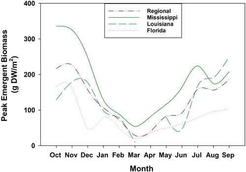
Table 2. Accumulated degree days (ADD) calculated for base temperatures of 0 and –6 °C (RMSE = 0.00) for each month from October 2021 to September 2022 for populations in Mississippi.

MONTH	ADD^a (base = 0 °C)	ADD (base = −6 °C)
October	404.7	584.25
November	653.45	1003.25
December	882.05	1410.7
January	1077.65	1743.6
February	1536.5	2387.4
March	2024.05	3054.15
April	2669.45	3885.55
May	3430.25	4826.35
June	4263.7	5845.8
July	5073.35	6835.45
August	5807.3	7755.4
September	6424.5	8558.6

^a ADD models predict 6469 ADD (292 calendar days) are needed for Cuban bulrush to reach peak biomass.

Table 3. Accumulated degree days (ADD) calculated for base temperatures of 0 and -3 °C (RMSE = 0.27) for each month from October 2021 to September 2022 for populations in Louisiana.

MONTH	ADD^a (base = 0^OC)	ADD (base = −3^OC)
October	727.5	820.5
November	1162.3	1371.95
December	1710.1	2035.85
January	2062.85	2456.5
February	2448.15	2894.5
March	2942.05	3497.8
April	3587.45	4216.8
May	4402.95	5125.3
June	5275.05	6087.4
July	6174.15	7079.5
August	7017.1	8044.3
September	7830.75	8919.1

^a ADD models predict 7903 ADD (331 calendar days) are needed for Cuban bulrush to reach peak biomass.

Table 4. Accumulated degree days (ADD) calculated for base temperatures of 0 and -2 °C (RMSE = 0.45) for each month from October 2021 to September 2022 for populations in Florida.

MONTH	ADD^a (base = 0^OC)	ADD (base = −2^OC)
October	591.4	651.4
November	967.5	1082.7
December	1367.35	1543.5
January	1813.25	2043.9
February	2378.95	2671.6
March	2957.5	3310.15
April	3669.95	4084.6
May	4466.1	4940.75
June	5309.8	5846.45
July	6140.05	6736.7
August	6943.3	7601.95
September	7643.55	8364.2

^a ADD models predict 7643 ADD (334 calendar days) are needed for Cuban bulrush to reach peak biomass.

Table 5. Accumulated degree days (ADD) calculated for base temperatures of 0 and -3 °C (RMSE = 0.18) for each month from October 2021 to September 2022 for a regional model that included sites from Mississippi, Louisiana, and Florida.

MONTH	ADD^a (base = 0^OC)	ADD (base = −3^OC)
October	327.88	416.23
November	655.93	836.70
December	957.52	1218.32
January	1482.7	1836.5
February	2031.63	2475.43
March	2727.93	3264.73
April	3520.55	4147.35
May	4373.77	5093.57
June	5236.65	6049.45
July	5989.63	6892.43
August	6671.28	7667.08
September	7121.23	8207.03

^a ADD models predict 7111 ADD (312 calendar days) are needed for Cuban bulrush to reach peak biomass.

Discussion

Current models estimated 6,469 ADD at a base threshold of −6 °C were needed to reach peak emergent Cuban bulrush biomass for plants growing in MS, 7,903 ADD at a base threshold of −3 °C for plants in LA, and 7,643 ADD at a base threshold of −2 °C for plants in FL. A previous study on Cuban bulrush estimated a base threshold temperature of −4 °C for plants in MS (Squires et al. 2024), which is similar to the model predictions from the current study. Notably populations in Mississippi were the monocephalous form whereas Louisiana and Florida populations were the polycephalous form, and a difference of almost 1,200 ADD and 3 °C (base threshold) was observed between the two Cuban bulrush forms. These results suggest that not only do environmental factors influence ADD modeling but biotype may also be important.

Temperature is a major driver of aquatic plant growth, and in most cases, warmer temperatures enhance plant growth and biomass accumulation (Wilson et al. 2005; Burnett et al. 2007). For instance, previous studies assessing the relationship of water hyacinth phenology and air temperature found a strong positive linear relationship between biomass and increasing air temperature (Wilson et al. 2005; Villamagna and Murphy 2010). Conversely, it was reported that Cuban bulrush growth was negatively correlated to water temperature, air temperature, and PAR with peak biomass occurring in February in populations from Mississippi (Clarke et al. 2023). Peak emergent biomass was recorded in September-October in the current study. However, higher total biomass in this study was recorded during colder months when average temperatures were 6.0 to 13.6 °C (December through January), 9.0 to 18.4 °C (December through January), and 14.2 to 17.3 °C (December through January) for Mississippi, Louisiana, and Florida, respectively. This suggests the observed peak growth for Cuban bulrush could shift temporally based on annual temperature cycles (e.g. warmer years vs. colder years). Furthermore, the base temperature thresholds generated from the current models suggest that Cuban bulrush is physiologically active at air temperatures below freezing. The tolerance to below freezing air temperatures may be an artifact of the latent heat of water, and water’s ability to resist major changes in temperature (Oke 1987). Thus, the water surrounding Cuban bulrush may allow for micro-climate moderation of atmospheric temperatures for a short time (Oke 1987; Burnett et al. 2007), thereby creating more optimal growing conditions for Cuban bulrush. The ability to grow in cooler temperatures may give Cuban bulrush a biological advantage, and could permit this species to dominate during times of lower temperatures where other plant species have decreased, or no, physiological activity (Clarke et al. 2023).

Predictions of plant growth based on ADD estimates can be useful in the development of landscape scale monitoring strategies to prevent further spread of invasive species. Such models have been used to predict sprouting and emergence of aquatic vegetative propagules for species like Hydrilla verticillata (L.f.) Royle, Potamogeton pectinatus L., Potomageton nodosus Poiret, and Vallisneria americana L. (Spencer et al. 2000; Spencer and Ksander 2006). However, as observed in Florida, states that have longer, less variable, or incremental growing seasons may not be suitable areas for estimating ADD requirements. For instance, Potamogeton crispus L. phenology is less incremental in Mississippi due to a longer growing season with less environmental cues than populations growing in Minnesota (Turnage et al. 2018; Woolf and Madsen 2003). This trend was also observed in long-leaf pondweed (Potamogeton nodosus) where biomass peaked earlier and more gradually in California compared to populations in Texas (Spencer et al. 2000).

Future models for Cuban bulrush growth should assess more sites across the invaded range including more populations of both Cuban bulrush forms and sites near the edge of the invasion front. Current models suggest that plants adapted to Florida conditions could spread as far north as Missouri based on the lower base temperature threshold (mean January temperature approximately −2 °C; National Centers for Environmental information 2023). Mississippi and Louisiana populations have the potential to spread as far north as Iowa (mean January temperature approximately −4 °C; NOAA 2023), though the main limiting factor in northern expansion will be prolonged ice cover on waterbodies. Future monitoring should prioritize states that may be at most risk of invasion (i.e. freshwater environments with temperatures above −6 °C and water that does not freeze throughout most of the winter months). Monitoring will become important as there is a predicted temperature increase of 2.7 C (4.9 °F) by the middle of this century (2046 to 2065) and 4.7 C (8.5 °F) by the end of the century (2081 to 2100) compared to temperatures recorded between 1979 and 2000 (Pryor et al. 2013). Consistent warmer temperatures would facilitate more rapid and wide spread geographic expansion of invasive species. Future efforts should also assess Cuban bulrush growth at temperatures around the base thresholds estimated in this study to gain a better understanding as to Cuban bulrush’s ability to grow in such temperatures, along with any climactic stressors, like snow or ice cover, that may be observed in the northern U.S.

Authors’ contributions

Gray Turnage and Ryan Wersal contributed to the study conception and design. Data collection was done by Allison Squires, Gray Turnage, Christopher Mudge, and Benjamin Sperry. Material preparation and analysis were performed by Gray Turnage, Ryan Wersal, and Allison Squires. The first draft of the manuscript was written by Allison Squires and all authors commented on previous versions of the manuscript. All authors read and approved the final manuscript.

Acknowledgements

The research was supported by the Aquatic Plant Control Research Program, U.S. Army Engineer Research & Development Center under cooperative agreement W912HZ2120036. The manuscript was reviewed in accordance with U.S. Army Engineer Research and Development Center policy and approved for publication. Citation of trade names does not constitute endorsement or approval of the use of such commercial products. The content of this work does not necessarily reflect the position or policy of the U.S. government and no official endorsement should be inferred. We would like to thank the USACE, Nature Conservancy, and Florida Fish and Wildlife Conservation Commission for allowing access to some of the field sites. We also thank Josh Long, Walt Maddox, Esther St. Pierre, Garret Ervin, Anna McLeod, Bram Finkle, and Graham Lightsey from Mississippi State University for technical assistance in field sampling and sample preparation. We thank Michael Durham of the University of Florida Center for Aquatic Invasive Plants for technical assistance in Florida. We thank David Sexton of the Louisiana State University Ag Center and Daniel Hill of the Louisiana Department of Wildlife and Fisheries for technical assistance in Louisiana. Lastly, we thank Max Gebhart and Hunter Kelzenberg from the Aquatic Weed Science Lab at Minnesota State University for sample preparation and analysis. This manuscript is a contribution of the Mississippi Agricultural and Forestry Experiment Station and the Mississippi Cooperative Extension Service.

Disclosure statement

No potential conflict of interest was reported by the author(s).

Data availability statement

Data are available from the authors upon reasonable request.

Additional information

Funding

Funding for this work was provided by a cooperative agreement (W912HZ-19-0003) from the Department of Defense U.S. Army Engineer Research and Development Center Aquatic Plant Control Research Program. The content of this work does not necessarily reflect the position or policy of the U.S. government and no official endorsement should be inferred.

References

- Arazi Y, Wolf S, Marani A. 1993. A prediction of developmental stages in potato plants based on the accumulation of heat units. Agric. Syst. 43(1):1–12. doi: 10.1016/0308-521X(93)90091-F.
- Barbosa AM, Brown JA, Jimenez-Valverde A, Real R. 2022. Package ‘modEvA’. R Package, Version 3.5. URL: https://cran.r-project.org/web/packages/modEvA/modEvA.pdf. Date accessed: 03-08-22.
- Bryson CT, Carter R. 2008. The significance of Cyperaceae as weeds. Monogr. Syst. Bot. Mo. Bot. Gard. 108:15–10.
- Bryson CT, Maddox VL, Carter R. 2008. Spread of Cuban club-rush (Oxycaryum Cubense) in the southeastern United States. Invasive Plant Sci. Manage. 1(3):326–329. doi: 10.1614/IPSM-08-083.1.
- Burnett DA, Champion PD, Clayton JS, Ogden J. 2007. A system for investigation of the temperature responses of emergent aquatic plants. Aquat. Bot. 86(2):187–190. doi: 10.1016/j.aquabot.2006.09.015.
- Carter R. 2005. An introduction to the sedges of Georgia. Tipularia. 20:15–44.
- Chapman AW. 1889. Flora of the southern states. 2nd ed. New York: Ivison, Blakeman and Company.
- Clarke M, Wersal RM, Turnage G. 2023. Seasonal phenology and starch allocation patterns of Cuban bulrush (Oxycaryum cubense) growing in Mississippi, USA. Aquat. Bot. 186:103627. doi: 10.1016/j.aquabot.2023.103627.
- Dancey CP, Reidy JG. 2004. Statistics Without Maths for Psychology: using SPSS for Windows. New York: Prentice Hall.
- Finch DM, Butler JL, Runyon JB, Fettig CJ, Kilkenny FF, Jose S, Frankel SJ, Cushman SA, Cobb RC, Dukes JS, et al. 2021. Effects of climate change on invasive species. In: Poland, TM, Patel-Weynand, T, Finch, DM, Miniat, CF, Hayes, DC, Lopez, VM, editors, Invasive Species in Forests and Rangelands of the United States. Cham: Springer. https://doi.org/10.1007/978-3-030-45367-1_4
- Forcella F, Banken KR. 1996. Relationships among green foxtail (Setaria viridis) seedling development, growing degree-days, and time of nicosulfuron application. Weed Technol. 10(1):60–67. doi: 10.1017/S0890037X00045711.
- Fox J, Weisberg S, Price B. 2022. Package ‘car’. R Package, Version 3.1-0. URL: https://cran.r-project.org/web/packages/car/car.pdf. Date accessed: 03-08-22.
- Grippo M, Fox L, Hayse J, Hlohowskyj I, Allison T. 2014. Risk of adverse impacts from the movement through the CAWS and establishment of aquatic nuisance species in the Great Lakes and Mississippi River basins. U. S. Army Corps of Engineers, Great Lakes and Mississippi River Inter Basin Study Final Report. Part 2: 410 pp. appendix E.
- Hayhoe HN, Dwyer LM. 1990. Relationship between percentage emergence and growing degree-days for corn. Can J Soil Sci. 70(3):493–497. doi: 10.4141/cjss90-048.
- Hosmer DW, Lemeshow S, Sturdivant RX. 2013. Applied Logistic Regression. Hoboken, NJ:Wiley.
- IPCC. 2022. Framing and context. In global warming of 1.5 °C: IPCC special report on impacts of global warming of 1.5 °C above pre-industrial levels in context of strengthening response to climate change, sustainable development, and efforts to eradicate poverty. p. 49–92. Cambridge: Cambridge University Press. doi: 10.1017/9781009157940.003.
- Kriticos DJ, Brunel S. 2016. Assessing and managing the current and future pest risk from water hyacinth, (Eichhornia crassipes), an invasive aquatic plant threatening the environment and water security. PLOS One. 11(8):e0120054. doi: 10.1371/journal.pone.0120054.
- Kuznetsova A, Brockhoff PB, Christensen RHB. 2020. Package ‘ImerTest’. R Package, Version 3.1-3. URL: https://cran.r-project.org/web/packages/lmerTest/lmerTest.pdf. Date accessed: 03-08-22.
- Lenth RV. 2022. Package ‘emmeans’. R Package, Version 1.7.5. URL: https://cran.r-project.org/web/packages/emmeans/emmeans.pdf. Date accessed: 03-08-22.
- Mangiafico S. 2022. Package ‘rcompanion’. R Package, Version 2.4.16. URL: https://cran.r-project.org/web/packages/rcompanion/rcompanion.pdf. Date accessed: 03-08-22.
- McFarland DG, Nelson LS, Grodowitz MJ, Smart RM, Owens CS. 2004. Salvinia molesta DS Mitchell (giant salvinia) in the United States: a review of species ecology and approaches to management (No. ERDC/EL-SR-04-2). US Army Corps of Engineers, Engineer Research and Development Center Vicksburg, MS Environmental Lab. :33. p.
- McMaster GS, Wilhelm W. 1997. Growing degree-days: one Equation, Two Interpretations. Publications from USDA-ARS/UNL Faculty. Paper 83. http://digitalcommons.unl.edu/usdaarsfacpub/83.
- (NOAA) National Centers for Environmental information. 2023. Climate at a glance: statewide mapping. In: National Climatic Data Center. National Oceanic and Atmospheric Administration, National Centers for Environmental Information. https://www.ncdc.noaa.gov/cag/statewide/mapping/110/tavg/202201/1/value. Accessed 01 Aug 2023.
- Nowosad J. 2021. Package ‘pollen’. R Package, Version 0.82.0. URL: https://cran.r-project.org/web/packages/pollen/pollen.pdf. Date accessed: 03-08-22.
- Ogle D, Doll J, Wheeler P, Dinno A. 2022. Package ‘FSA’. R Package, Version 0.9.3. URL: https://cran.r-project.org/web/packages/FSA/FSA.pdf. Date accessed: 03-08-22.
- Oke TR. 1987. Boundary layer climates. London England: Routledge,.
- Pinheiro J, Bates D. 2022. Package ‘nlme’. R Package, Version 3.1-158. URL: https://cran.r-project.org/web/packages/nlme/nlme.pdf. Date accessed: 03-08-22.
- Pruim R, Kaplan DT, Horton NJ. 2021. Package ‘mosaic’. R Package, Version 1.8.3. URL: https://cran.r-project.org/web/packages/mosaic/mosaic.pdf. Date accessed: 03-08-22.
- Pryor S, Barthelmie R, Schoof J. 2013. High-resolution projections of climate-related risks for the Midwestern USA. Clim Res. 56(1):61–79. doi: 10.3354/cr01143.
- R Core Team. 2022. R: a language and environment for statistical computing. R Foundation for Statistical Computing, Vienna, Austria. www.R-project.org/.
- Revelle W. 2022. Package ‘psych’. R Package, Version 2.2.5. URL: https://cran.r-project.org/web/packages/psych/psych.pdf. Date accessed: 03-08-22.
- Riis T, Olesen B, Clayton J, Lambertini C, Brix H, Sorrell B. 2012. Growth and morphology in relation to temperature and light availability during the establishment of three invasive aquatic plant species. Aquat. Bot. 102:56–64. doi: 10.1016/j.aquabot.2012.05.002.
- Ritz C, Strebig JC. 2016. Package ‘drc’. R Package, Version 3.0-1. URL: https://cran.r-project.org/web/packages/drc/drc.pdf. Date accessed: 03-08-22.
- Robinson D, Hayes A, Couch S. 2022. Package ‘broom’. R Package, Version 1.0.0. URL: https://cran.r-project.org/web/packages/broom/broom.pdf. Date accessed: 03-08-22.
- Roltsch WJ, Zalom FG, Strawn AJ, Strand JF, Pitcairn MJ. 1999. Evaluation of several degree-day estimation methods in California climates. Inter. J. Biometeor. 42(4):169–176. doi: 10.1007/s004840050101.
- Sanderson MA, Karnezo TP, Matches AG. 1994. Morphological development of alfalfa as a function of degree-days. J. Product. Agric. 7(2):239–242. doi: 10.2134/jpa1994.0239.
- Sartain BT, Turnage G, Madsen JD. 2014. Aquatic plant community and invasive plant management assessment of the Ross Barnett reservoir, MS in 2013. Geosystems Res Inst Report. 5062:34 p.
- SERNEC. 2022. Southeastern regional network of expertise and collections. http://sernecportal.org/portal/collections/index.php. Accessed 24 May 2023.
- Snyder R. 1985. Hand calculating degree-days. Agric. For. Meteorol. 35(1–4):353–358. doi: 10.1016/0168-1923(85)90095-4.
- Snyder RL, Spano D, Cesaraccio C, Duce P. 1999. Determining degree-day thresholds from field observations. Int. J. Biometeorol. 42(4):177–182. doi: 10.1007/s004840050102.
- Spencer DF, Ksander GG, Madsen JD, Owens CS. 2000. Emergence of vegetative propagules of Potamogeton nodosus, Potamogeton pectinatus, Vallisneria Americana, and Hydrilla verticillata based on accumulated degree-days. Aquat. Bot. 67(3):237–249. doi: 10.1016/S0304-3770(00)00091-7.
- Spencer DF, Ksander GG. 2006. Estimating Arundo donax ramet recruitment using degree-day-based equations. Aquat. Bot. 85(4):282–288. doi: 10.1016/j.aquabot.2006.06.001.
- Squires AC, Turnage G, Wersal RM. 2024. Modeling accumulated degree-days for the invasive aquatic plants Oxycaryum cubense and Eichhornia crassipes in Mississippi. J. Aquat. Plant Manage. 62:23–29 doi: 10.57257/JAPM-D-23-00006.
- Turnage G, Madsen JD, Wersal RM. 2018. Phenology of curlyleaf pondweed (Potamogeton crispus L.) in the southeastern United States: a two-year mesocosm study. J. Aquat. Plant Manage. 56:35–38.
- Turnage G, Shoemaker C. 2017. 2017 Survey of aquatic plant species in Mississippi waterbodies. Geosystems Res Inst Report. 5077:69 p.
- UC IPM. 2016. About Degree-Days. In: how to Manage Pests: degree Days. Agriculture and Natural Resources, University of California. https://ipm.ucanr.edu/WEATHER/ddconcepts.html.
- Villamagna AM, Murphy BR. 2010. Ecological and socio-economic impacts of invasive E. crassipes (Eichhornia crassipes): a review. Freshw. Biol. 55(2):282–298. doi: 10.1111/j.1365-2427.2009.02294.x.
- Vose RS, Easterling DR, Kunkel KE, LeGrande AN, Wehner MF. 2017. Temperature changes in the United States. In: Wuebbles, DJ, Fahey, DW, Hibbard, KA, Dokken, DJ, Stewart, BC, Maycock, TK, editors. Climate Science Special Report: Fourth National Climate Assessment. U.S. Global Change Research Program; Vol. 1, p. 185–206. doi: 10.7930/J0N29V45.
- Watson AL, Madsen JD. 2014. The effect of the herbicide and growth stage on Cuban club-rush (Oxycaryum cubense) control. J Aquat. Plant Manage. 52:71–74.
- Wickham H, Hester J, Chang W, Bryan J. 2022. Package ‘devtools’. R Package, Version 2.4.4. URL: https://cran.r-project.org/web/packages/devtools/devtools.pdf. Date accessed: 03-08-22.
- Wickham H. 2022. Package ‘tidyverse’. R Package, Version 1.3.2. URL: https://cran.r-project.org/web/packages/tidyverse/tidyverse.pdf. Date accessed: 03-08-22.
- Wilson JR, Holst N, Rees M. 2005. Determinants and patterns of population growth in E. crassipes. Aquat. Bot. 81(1):51–67. doi: 10.1016/j.aquabot.2004.11.002.
- Woolf TE, Madsen JD. 2003. Seasonal biomass and carbohydrate allocation patterns in southern Minnesota curlyleaf pondweed populations. J. Aquat. Plant Manage. 41:113–118.
- Yang S, Logan J, Coffey DL. 1994. Mathematical formulae for calculating the base temperature for growing degree days. Agri. Forest Meteor. 74(1-2):61–74. doi: 10.1016/0168-1923(94)02185-M.
- Zalom F, Goodell P, Wilson L, Barnett WW, Bentley WJ. 1983. Degree-Days, the Calculation and Use of Heat Units in Pest Management: University of California Division of Agriculture and Natural Resources Leaflet 21373. Berkeley: University of California.