Loss modeling with many-parameter distributions

Abstract

It is argued that many-parameter families of loss distributions may work even with limited amounts of historical data. A restriction to unimodality works as a stabilizer, which makes fitted distributions much more stable than their parameters. We propose Box-Cox transformed Gamma and Burr variables. Those are models with three or four parameters with many of the traditional two-parameter families as special cases, and there are well-defined distributions at the boundaries of the parameter space, which is important for stability. The approach is evaluated with model error defined though the theory of misspecification in statistics. It is shown that such error is drastically reduced when a third or fourth parameter is added without increasing the random error more than a little. It is pointed out that the approach may be a suitable starting point for completely automatic procedures.

Keywords:

• Asymptotics
• Box-Cox transformation
• Burr distribution
• insurance claims
• misspecified model
• reserve estimate

1. Introduction

Modeling insurance losses from historical observations might have been carried out by the empirical distribution or by non-parametric density estimation (for example Scott 1992) if it had not been for future, huge losses not in the data. Indeed, the importance of this extreme right tail has promoted special methods to deal with it; Embrechts et al. (1997) is the standard reference. Yet, in practical insurance, two-parameter models is without doubt still one of the most common approaches (Omari et al. 2018). The drawback is that distributions now are tied to a specific shape for which there may be little theoretical justification. Families of distributions with more than two parameters such as the Burr family which goes back to Burr (1942) or the transformed Beta and Gamma distributions in Venter (1985), also treated in Kleiber & Kotz (2003) and Cummins et al. (1990), would be more flexible. It is the aim of the present paper to argue for the use of such multi-parameter families among which we construct a new one with attractive properties. Another tradition in actuarial science is to use slicing or composite distributions with different parametric families imposed on each side of a threshold. The approach has some support in Pickands' theorem, which reveals that tail distributions always become Pareto or exponentially distributed when the threshold tends to infinity. The problem here is that it varies enormously from case to case how large the threshold must be; see Bølviken (2014). This motivates other composite models, and they have in recent years been proposed in large numbers, see for example Cooray & Ananda (2005), Scollnik (2007), Scollnik & Sun (2012), Bakar et al. (2015), Reynkens et al. (2017) and Chan et al. (2018). Composites can be seen as special cases of mixture distributions which have also been used for loss modeling. Some references are Lee & Lin (2010), Verbelen et al. (2015), Miljkovic & Grün (2016) and Gui et al. (2021).

The key issue is how to cope with a lack of knowledge of the shape of the underlying distribution when the experience to go on is limited. One approach, used in Miljkovic & Grün (2016), is to try several families of distributions and select the best-fitting one, another is the so-called Bayesian averaging in Hoeting et al. (1999). Still another, and in our view simpler way, is to start out with multi-parameter models containing the standard two-parameter ones as special cases. There are several possibilities (see above), but our preferred vehicle is the Box-Cox-transformed Gamma and Burr variables constructed in the next section. These models are always unimodal to which we attach great importance. Is such a delimitation too narrow in scope?

Loss data from different populations is common, but their origin would often be known, and we are then in a regression situation outside the realm of this paper. Mixture distributions arise when the underlying populations are unobservable or latent so that it is not known which populations individual losses come from. Whether this violates unimodality depends on how far apart the populations are, but even if multimodality would have been spotted with lots of data, it might not be for smaller amounts. Further, there is a price to be paid for all this flexibility; it is bound to make modeling more vulnerable to random error. This is demonstrated by example in Section 4, and that is where our idea kicks off. By imposing unimodality, fitted distributions might be stable even when there are many parameters and not overwhelmingly much data. The rationale is as follows. Many-parameter, unimodal families will inevitably contain distributions resembling each other, which can only mean uncertain parameter estimates. However, those are not really the target, and the fitted distributions they lead to are much less vulnerable to random error. The transformation families proposed in Section 2 work not only because their distributions are unimodal, but also because they tend to well-defined distributions at the boundary of the parameter space, which is important for their behavior when fitted. This makes it possible to program automatic methods where the computer on its own picks a distribution from the three- or four-parameter family, without human intervention, thus avoiding the whole model selection step, which is particularly useful when data are not abundant.

Then the question is how different methods should be evaluated and compared. What really matters is not the loss model itself, but rather its impact on what it is used for, for example on the projected reserve of a portfolio, which is the chief criterion in the remains of the paper. There are both modeling and sampling error to deal with, and one way to make the distinction between them precise is to draw on the asymptotic theory of likelihood estimates in misspecified models; White (1982) is a much cited reference. Suppose a family of distributions parameterized by θ has been imposed with $\hat{\theta }$ its likelihood estimate. As the number of historical losses become infinite, $\hat{\theta }$ will nearly always converge to some ${\theta }^{\ast }$ even if the true loss distribution is outside the family. This ${\theta }^{\ast }$-distribution minimizes the so-called Kullback-Leibler distance to the true one (Section 2.4), and provides a reasonable definition of model error. When we in Section 2.5 compare the projected reserve under these two distributions over a broad range of possibilities, it will emerge that a third parameter often lowers model error drastically and that a fourth one makes it very small indeed.

Model error under our transformation models is thus fairly small, but then there is random error, which we study by both asymptotics and Monte Carlo. One side of that is over-parameterization; how much extra random error is brought in when extra parameters are added, for instance to a two-parameter family? Special weight is placed on log-normal models under which error studies can be carried out by particularly simple mathematics. One thing that must be kept in mind is that errors with scarce data and heavy-tailed distributions might be large in any case, and the real question is how much larger they become when additional parameters are added. Bayesian assumptions if warranted might mitigate error, but that is outside the scope of this paper.

The outline of this paper is as follows. Multi-parameter modeling and model misspecification are introduced in Section 2. Section 3 presents asymptotic results concerning the error that is made using a multi-parameter model when the true model is a simpler one, whereas this is explored in a simulation study in Section 4. An illustrative example involving Norwegian automobile insurance losses is given in Section 5. Finally, Section 6 contains some concluding remarks.

2. A multi-parameter approach

2.1. The Burr model

One way of defining families of loss distributions beyond the two-parameter ones is through ratios of Gamma variables (Venter 1985, Kleiber & Kotz 2003). Let (1) $X=\frac{G_{\theta }}{G_{\alpha }}$(1) with $G_{\alpha }$ and $G_{\theta }$ two independent Gamma variables with mean 1 and shape α and θ. This is the Burr model, also called Beta Prime, Pearson type 6 and extended Pareto, which goes back to Burr (1942). It can also be defined through its density function (2) $f\left(x\right)=\frac{\mathrm{\Gamma }(\alpha +\theta )}{\mathrm{\Gamma }\left(\alpha \right)\mathrm{\Gamma }\left(\theta \right)}{\left(\frac{\alpha }{\theta }\right)}^{\alpha }\frac{x^{\theta -1}}{(\alpha /\theta +x{)}^{\alpha +\theta }},x>0.$(2) Adding a parameter of scale $\text{β}>0$ leads to a model $Z=\text{β}X$ for a claim Z. Its moments are (3) $E\left(Z^k\right)={\left(\frac{\alpha }{\theta }\right)}^k\left(\prod _{j=1}^k\frac{\theta +j-1}{\alpha -j}\right){\text{β}}^k,k=1,2,\dots$(3) which are finite when $k<\alpha$.

One of the attractive sides of this framework is that it captures under the same roof both heavy-tailed Pareto distributions when $\theta =1$ and more light-tailed Gamma ones which appear when $\alpha \to \mathrm{\infty }$. The latter is an immediate consequence of (1(1) $X=\frac{G_{\theta }}{G_{\alpha }}$(1) ) since $G_{\alpha }\stackrel{p}{\to }1$ as $\alpha \to \mathrm{\infty }$ by virtue of $E\left(G_{\alpha }\right)=1$ and sd$\left(G_{\alpha }\right)=1/\sqrt{\alpha }$, and a similar argument shows that the inverse Gamma $1/G_{\alpha }$ emerges when $\theta \to \mathrm{\infty }$.

2.2. Transformation modeling

One way to extend the Burr family is to use parameterized transformations, say (4) $Z=\text{β}h(X;\eta )$(4) with $\eta >0$ an additional parameter and $h(x;\eta )$ some increasing function to be specified. An example of such a construction is the generalized beta distribution of order II (GB2), that uses $h(x;\eta )=x^{1/\eta }$ which is mentioned in Kleiber & Kotz (2003) (see p. 190), and used for modeling insurance losses in Cummins et al. (1990).

A natural restriction is $h(x;1)=x$, making the Burr model a special case. Not all functions $h(x;\eta )$ satisfying these conditions lead to the families of unimodal distributions, but one possibility is the Box-Cox transformation $h(x;\eta )=(1+x{)}^{\eta }-1$ which goes back to Box & Cox (1964). This choice sets up what we shall refer to as the PowerGamma and PowerBurr models (5) $Z=\text{β}\left\{\right(1+G_{\theta }{)}^{\eta }-1\}\text{and}Z=\text{β}\{(1+X{)}^{\eta }-1\}$(5) with parameters θ, η and β for PowerGamma on the left and α, θ, η and β for PowerBurr on the right. The latter collapses to PowerGamma when $\alpha \to \mathrm{\infty }$. It will emerge in Section 3 that the log-normal is a special case of both, and most other standard loss models are included approximately. The PowerGamma and PowerBurr families are unimodal everywhere; i.e. their density functions are monotonely decreasing when $\theta \le 1$ and have a single maximum otherwise, which follows easily from their mathematical expressions in Appendices C and D.

One of the attractive features of the Box-Cox transformation is its behavior as $\eta \to 0$. It follows from (5(5) $Z=\text{β}\left\{\right(1+G_{\theta }{)}^{\eta }-1\}\text{and}Z=\text{β}\{(1+X{)}^{\eta }-1\}$(5) ) that $Z=\text{β}\mathrm{\eta log}(1+G_{\theta })+o_p\left(\eta \right)$ on the left and $Z=\text{β}\mathrm{\eta log}(1+X)+o_p\left(\eta \right)$ on the right, in both cases in the limit well-defined models with scale parameter $\text{β}\eta$. We believe this property to have a stabilizing influence when models are fitted. Indeed, it is worth recording what happens with the perhaps superficially equally attractive $h(x;\eta )=x^{\eta }$. The models for $Z=\text{β}{G}_{\theta }^{\eta }$ and $Z=\text{β}{X}^{\eta }$ are again unimodal, but now (for example) $\text{β}{X}^{\eta }=\text{β}+\text{β}\mathrm{\eta log}\left(X\right)+o_p\left(\eta \right)$ as $\eta \to 0$, and a very small η can only be compensated by extreme variation in X. Such solutions simply are not plausible, yet likelihood fitting for moderate or small amounts of data often came up with them when the transformation was tried out. Does a restriction such as $\eta \ge 1$ get rid of them? The problem is that these freak solutions now turn into η-estimates close to 1, and such fitting when examined implied considerable estimation bias, in the sense that the estimated distribution did not fit the data well.

2.3. Illustration

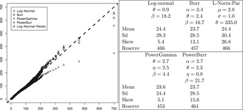
A small example of how such modeling may work is shown in Table 1 where the Gamma, Pareto, Burr, PowerGamma and PowerBurr distributions have been fitted the n = 60 Belgian fire losses from Beirlant et al. (1996), here scaled so their average is one (R-code for fitting the Burr, PowerGamma and PowerBurr is available in https://github.uio.no/ingrihaf/PowerBurr). The parameter values from the five fitted distributions are displayed along with the corresponding means, standard deviations and skewnesses. We have also computed the $99\mathrm{\%}$ reserve of a portfolio, i.e. the $99\mathrm{\%}$ percentile of the distribution of the total portfolio loss. We assumed a Poisson distribution for the number of claims with expectation $\lambda =10$, and each of the five distributions as the claim size distribution. The resulting reserves are shown in the rightmost column of the Table. Not all modeling based on 60 losses can be expected to be as stable, with standard deviations, skewnesses and reserves that hardly vary with the different loss models. The very large α for Burr and PowerBurr ($\mathrm{22,000}$ was the maximum value allowed) signify that $G_{\alpha }\approx 1$ in (1(1) $X=\frac{G_{\theta }}{G_{\alpha }}$(1) ), so that the Burr and the PowerBurr models obtained are very nearly Gamma and PowerGamma. Standard deviations match the empirical one in the data, which is 1.02, whereas the skewness is substantially higher than the empirical skewness coefficient of 1.46, but which is known to under-estimate the true skewness; see for instance Bølviken (2014).

Table 1. Parameters, mean, sd, skewness and $99\mathrm{\%}$ reserve for the Belgian fire data.

	α	β	θ	η	$E\left(Z\right)$	sd(Z)	skew(Z)	reserve
Gamma		1.00	0.90		1.00	1.05	2.11	22.9
Pareto	33.5	0.97			1.00	1.03	2.19	22.8
Burr	22,000	1.00	0.90		1.00	1.06	2.11	22.9
PowerGamma		1.00	0.90	1.00	1.00	1.06	2.11	22.9
PowerBurr	22,000	1.00	0.90	1.00	1.00	1.04	2.02	22.9

Note: with the reserve computed by Monte Carlo (one million simulations)

2.4. Misspecification

Let $f(z;\mathbf{p})$ be the density function of Z under one of the models above depending on the parameter vector $\mathbf{p}$, and let ${\hat{\mathbf{p}}}_n$ be the maximum likelihood estimate of $\mathbf{p}$ based on n historical losses. Maximum likelihood is not only the standard method, but also has an appealing error theory. Suppose the true density function $g\left(z\right)$ differs from $f(z;\mathbf{p})$ for all $\mathbf{p}$. Such model error is highly relevant in insurance since there is typically little hard justification for the parametric families imposed. However, even when they do not contain the true distribution, there usually exists some ${\mathit{p}}^{\ast }$ so that ${\hat{\mathbf{p}}}_n\stackrel{p}{\to }{\mathbf{p}}^{\ast }$ as $n\to \mathrm{\infty }$. Indeed, it was shown in Huber (1967) and later in White (1982, 1994) under very general conditions that ${\mathbf{p}}^{\ast }$ minimizes the Kullback-Leibler divergence of the family $f(z;\mathbf{p})$ with respect to the true $g\left(z\right)$, i.e. (6) $\mathcal{E}(\mathbf{p};g)={\int }_0^{\mathrm{\infty }}\log \frac{g\left(z\right)}{f(z;\mathbf{p})}g\left(z\right)\mathrm{d}z.$(6) If $g\left(z\right)=f(z;\mathbf{p})$ for some $\mathbf{p}$, then ${\mathbf{p}}^{\ast }=\mathbf{p}$, but otherwise $f(\mathbf{z};{\mathbf{p}}^{\ast })$, minimizing (6(6) $\mathcal{E}(\mathbf{p};g)={\int }_0^{\mathrm{\infty }}\log \frac{g\left(z\right)}{f(z;\mathbf{p})}g\left(z\right)\mathrm{d}z.$(6) ), deviates from the true $g\left(z\right)$, resulting in model error.

Consider a quantity of interest ψ, for example the reserve of a portfolio in general insurance, i.e. a percentile of the total loss distribution, and write $\psi \left(\mathbf{p}\right)$ for its value when $f(z;\mathbf{p})$ is the loss distribution. The value we seek is $\psi \left(g\right)$ under the true density function $g\left(z\right)$, whereas our estimate is $\psi \left({\hat{\mathbf{p}}}_n\right)$, and its error can be decomposed as (7) $\psi \left({\hat{\mathbf{p}}}_n\right)-\psi \left(g\right)=\psi \left({\hat{\mathbf{p}}}_n\right)-E\left\{\psi \right({\hat{\mathbf{p}}}_n\left)\right\}+E\left\{\psi \right({\hat{\mathbf{p}}}_n\left)\right\}-\psi \left(g\right),$(7) where the first component on the right reflects the standard error of the estimate. The second component is bias which is the sum of two contributions; i.e. (8) $E\left\{\psi \right({\hat{\mathbf{p}}}_n\left)\right\}-\psi \left({\mathbf{p}}^{\ast }\right)+\psi \left({\mathbf{p}}^{\ast }\right)-\psi \left(g\right)$(8) with model error on the right which is what remains when $n\to \mathrm{\infty }$. There is no such error when the PowerGamma or the PowerBurr models from Section 2.1 are fitted Gamma, Pareto or log-normal data.

2.5. Model error

To examine the model error numerically, consider the computation of the reserve in a small Poisson portfolio in general insurance with $\lambda =10$ expected events, meaning a percentile of the total portfolio loss distribution. The true loss models are varied among four different families, notably the log-normal $Z=\text{β}{\mathrm{e}}^{\mathrm{\theta Y}}$ with $Y\sim N(0,1)$, the log-Gamma $Z=\text{β}({\mathrm{e}}^{G_{\theta }}-1)$ where $G_{\theta }$ is a Gamma-variable with mean 1 and shape θ, the Weibull model $Z=\text{β}{G}_1^{1/\theta }$ and the logistic distribution defined by $\text{Pr}(Z\le z)=1-1/(1-\theta +\theta {\mathrm{e}}^{z/\text{β}})$ with $0<\theta \le 1$. The reserve was computed assuming each of the loss models Pareto, Burr, PowerGamma and PowerBurr in addition to the true one. In the cases where the assumed distribution $f(z;\mathbf{p})$ did not include the true distribution $g\left(z\right)$ as a special case, the best-fitting parameter vector ${\mathbf{p}}^{\ast }$ was found by minimizing the Kullback-Leibler divergence (6(6) $\mathcal{E}(\mathbf{p};g)={\int }_0^{\mathrm{\infty }}\log \frac{g\left(z\right)}{f(z;\mathbf{p})}g\left(z\right)\mathrm{d}z.$(6) ) numerically. Finally Monte Carlo with ten million simulations were used to calculate the $99\mathrm{\%}$ reserve under the true $g\left(z\right)$ and the approximating one $f(z;{\mathbf{p}}^{\ast })$.

Table 2 reports how much the reserve changes (in per cent) when $g\left(z\right)$ is replaced by the best-fitting $f(z;{\mathbf{p}}^{\ast })$. In mathematical terms the criterion is $\left(\psi \right({\mathbf{p}}^{\ast }\left)/\psi \right(g)-1)\times 100,$$\psi (\cdot )$ being the reserve, which does not depend on β so that only the shape parameter θ has to be varied. Their values in Table 2 have been chosen with some care to reflect a reasonable range of skewness. The log-Gamma distribution is so heavy-tailed at $\theta =1$ or lower that not even the expectation is finite, and both the log-normal with $\theta =1$ and the Weibull distribution with $\theta =0.5$ allow very large claims. The results show how well higher-parameter distributions approximate many standard models. Whereas two-parameter Pareto fitting (included for comparison) over-shoots the target enormously, the four-parameter PowerBurr has inconsequential model bias everywhere, and also the three-parameter PowerGamma, except for the exceptionally heavy-tailed log-Gamma case with $\theta =1$. Unlike the other fitted distributions, the PowerGamma does not contain the Pareto family as a special case, but when model bias was calculated as described above, it was again largely minor; i.e. $-1.1\mathrm{\%}$ when the Pareto parameter $\alpha =10$, $-3.5\mathrm{\%}$ when $\alpha =5$ and $-27.2\mathrm{\%}$ when $\alpha =2$, the latter so heavy-tailed that the variance is infinite.

Table 2. Model bias in the estimated $99\mathrm{\%}$ reserve in $\mathrm{\%}$ of the true values under Pareto Burr, PowerGamma and PowerBurr fitting.

	Log-normal			Log-gamma
Model fitted	$\theta =0.2$	$\theta =0.5$	$\theta =1$	$\theta =1$	$\theta =5$	$\theta =10$
Pareto	22.8	15.0	−8.1	360	−6.0	14.2
Burr	−0.1	0.2	10.5	0.2	0.4	0.0
PowerGamma	0	0	0	−73.2	−3.9	−0.4
PowerBurr	0	0	0	−2.1	−0.3	−0.1
	Weibull			Logistic
Model fitted	$\theta =0.5$	$\theta =0.67$	$\theta =3$	$\theta =0.05$	$\theta =0.5$	$\theta =0.95$
Pareto	huge	5511	9.4	16.8	5.7	0.5
Burr	26.5	5.8	0.6	2.4	2.0	0.2
PowerGamma	1.2	0.3	−0.2	0.0	−0.4	0.1
PowerBurr	1.6	0.7	−0.0	−0.3	−0.1	0.0

3. Over-parameterization

3.1. Introduction

Modeling beyond two parameters introduces extra parameter uncertainty if one of the usual two-parameter sub-families is the true one. The size of the degradation can be explored analytically through asymptotics as $n\to \mathrm{\infty }$. Let $\mathit{p}=(p_1,\dots ,p_d)$ be the parameter vector and consider moments ${\mu }_k\left(\mathit{p}\right)=E(Z^k;\mathit{p})$ and percentiles $q_{ϵ}\left(\mathit{p}\right)$ defined as Pr$(Z\le q_{ϵ}(\mathit{p});\mathit{p})=ϵ$. Their estimates are ${\hat{\mu }}_{\mathrm{kn}}={\mu }_k\left({\hat{\mathit{p}}}_n\right)$ and ${\hat{q}}_{\mathrm{ϵn}}=q_{ϵ}\left({\hat{\mathit{p}}}_n\right)$ where ${\hat{\mathit{p}}}_n$ is the maximum likelihood estimate of $\mathit{p}$ based on n observations of Z.

Under the assumption that the model $f(z;\mathit{p})$ is the true one, theoretical statistics offer an approximation of $\text{sd}\left({\hat{\mu }}_{\mathrm{kn}}\right)$ and $\text{sd}\left({\hat{q}}_{\mathrm{ϵn}}\right)$ through the information matrix $I=\left(I_{\mathrm{ij}}\right)$ and the gradient vectors ${\mathit{v}}_k=\left(v_{\mathrm{ki}}\right)$ for ${\mu }_k\left(\mathit{p}\right)$ and ${\mathit{v}}_{ϵ}=\left(v_{\mathrm{ϵi}}\right)$ for $q_{ϵ}\left(\mathit{p}\right)$, where (9) $I_{\mathrm{ij}}=E\left(\frac{\mathrm{\partial }\log \left\{f\right(Z;\mathit{p})}{\mathrm{\partial }{p}_i}\frac{\mathrm{\partial }\log \left\{f\right(Z;\mathit{p})}{\mathrm{\partial }{p}_j}\right),v_{\mathrm{ki}}=\frac{\mathrm{\partial }{\mu }_k\left(\mathbf{p}\right)}{\mathrm{\partial }{p}_i}\text{and}{v}_{\mathrm{ϵi}}=\frac{\mathrm{\partial }{q}_{ϵ}\left(\mathbf{p}\right)}{\mathrm{\partial }{p}_i},i,j=1,\dots ,d.$(9) For moment estimation the result is (10) $\text{sd}\left({\hat{\mu }}_{\mathrm{kn}}\right)=\frac{s_k\left(\mathit{p}\right)}{\sqrt{n}}+o\left(1\sqrt{n}\right),s_k\left(\mathit{p}\right)=\sqrt{{{\mathit{v}}_k}^T{I}^{-1}{\mathit{v}}_k}.$(10) For percentile estimation the results is the same except for $s_k\left(\mathit{p}\right)$ being replaced by $s_{ϵ}\left(\mathit{p}\right)=\sqrt{{{\mathit{v}}_{ϵ}}^T{I}^{-1}{\mathit{v}}_{ϵ}}$.

A more general form, replacing the information matrix with a sandwich form, covers the situation when the model is misspecified, consult White (1982). Such an extension is relevant for the problems under discussion here, but we shall make no use of it. Our aim in this section is to evaluate $s_k\left(\mathit{p}\right)$ under a default, two-parameter model and examine how much it increases when a wider three or four-parameter one is being used.

How large n must be for the asymptotic results to be reasonably accurate approximations in the finite sample case was checked by Monte Carlo and varied with both the skewness of the distribution and with the quantity estimated. In Tables 3 and 4 below, n = 100 observations or even lower (n = 50) are often enough to get rather accurate results with the asymptotic formulas. The convergence is faster for the percentiles than the higher order moments and becomes slower when skewness is high.

Table 3. Relative increase (in $\mathrm{\%}$) in the asymptotic standard error of moment and percentile estimates when Burr has been fitted Pareto and Gamma data.

		Moments estimated			Percentiles estimated
True family of distributions		$E\left(Z\right)$	$E\left(Z^2\right)$	$E\left(Z^3\right)$	$50\mathrm{\%}$	$95\mathrm{\%}$	$99.5\mathrm{\%}$
	$\alpha =5$	0.1	2.5	8.1	0.0	0.1	4.1
Pareto	$\alpha =10$	0.0	0.6	3.6	0.1	0.5	3.5
	$\alpha =100$	0.0	0.0	1.0	0.4	1.0	2.7
	$\theta =1$	0.0	6.8	28.3	7.6	3.7	63.7
Gamma	$\theta =10$	0.0	0.3	1.9	8.0	8.8	58.6
	$\theta =100$	0.0	0.0	0.3	8.0	9.6	52.5

Table 4. Relative increase (in $\mathrm{\%}$) in asymptotic standard error of moment and percentile estimates when PowerGamma has been fitted log-normal data.

		Moment estimates			Percentile estimates
True family of distributions		$E\left(Z\right)$	$E\left(Z^2\right)$	$E\left(Z^3\right)$	$50\mathrm{\%}$	$95\mathrm{\%}$	$99.5\mathrm{\%}$
	$\sigma =0.25$	0.0	0.5	2.0	8.0	9.8	49.2
Log-normal	$\sigma =0.5$	0.0	5.4	18.2	8.0	9.8	49.2
	$\sigma =1.0$	5.4	37.4	85.9	8.0	9.8	49.2

3.2. Burr against Pareto and Gamma

The first example examines how much Burr fitting inflates uncertainty when the data come from a Pareto or a Gamma distribution. Write the coefficients $s_k\left(\mathit{p}\right)$ and $s_{ϵ}\left(\mathit{p}\right)$ in (10(10) $\text{sd}\left({\hat{\mu }}_{\mathrm{kn}}\right)=\frac{s_k\left(\mathit{p}\right)}{\sqrt{n}}+o\left(1\sqrt{n}\right),s_k\left(\mathit{p}\right)=\sqrt{{{\mathit{v}}_k}^T{I}^{-1}{\mathit{v}}_k}.$(10) ) as $s_k^{\text{bu}}(\alpha ,\theta ,\text{β})$ and $s_{ϵ}^{\text{bu}}(\alpha ,\theta ,\text{β})$ under the Burr model and $s_k^{\text{pa}}(\alpha ,\text{β})$ and $s_{ϵ}^{\text{pa}}(\alpha ,\text{β})$ under Pareto. The latter is the special case $\theta =1$, and the ratios $s_k^{\text{bu}}(\alpha ,1,\text{β})/s_k^{\text{pa}}(\alpha ,\text{β})$ and $s_{ϵ}^{\text{bu}}(\alpha ,1,\text{β})/s_{ϵ}^{\text{pa}}(\alpha ,\text{β})$ indicate extra uncertainty when the Burr family is fitted to Pareto data. We have chosen to report (11) $D_k^{\mathrm{bu}|\mathrm{pa}}(\alpha ,\text{β})=\frac{s_k^{\mathrm{bu}}(\alpha ,1,\text{β})}{s_k^{\mathrm{pa}}(\alpha ,\text{β})}-1\text{and}{D}_{ϵ}^{\mathrm{bu}|\mathrm{pa}}(\alpha ,\text{β})=\frac{s_{ϵ}^{\mathrm{bu}}(\alpha ,1,\text{β})}{s_{ϵ}^{\mathrm{pa}}(\alpha ,\text{β})}-1,$(11) the degree of degradation under Burr. Mathematical expressions for the information matrix I and the gradient vector ${\mathit{v}}_k$ under the Burr and the Pareto are given in Appendix A.

When the Gamma distribution replaces the Pareto as the true, data generating model, there is the slight complication that the true model now is on the boundary of the parameter space since Burr tends to Gamma as $\alpha \to \mathrm{\infty }$. The degree of degradation thus becomes (12) $D_k^{\mathrm{bu}|\mathrm{ga}}(\theta ,\text{β})=\frac{\underset{\alpha \to \mathrm{\infty }}{lim}{s}_k^{\mathrm{bu}}(\alpha ,\theta ,\text{β})}{s_k^{\mathrm{ga}}(\theta ,\text{β})}-1\text{and}{D}_{ϵ}^{\mathrm{bu}|\mathrm{ga}}(\theta ,\text{β})=\frac{\underset{\alpha \to \mathrm{\infty }}{lim}{s}_{ϵ}^{\mathrm{bu}}(\alpha ,\theta ,\text{β})}{s_{ϵ}^{\mathrm{ga}}(\theta ,\text{β})}-1$(12) with $s_k^{\text{ga}}(\theta ,\text{β})$ and $s_{ϵ}^{\text{ga}}(\theta ,\text{β})$ the coefficients $s_k\left(\mathit{p}\right)$ and $s_{ϵ}\left(\mathit{p}\right)$ in (10(10) $\text{sd}\left({\hat{\mu }}_{\mathrm{kn}}\right)=\frac{s_k\left(\mathit{p}\right)}{\sqrt{n}}+o\left(1\sqrt{n}\right),s_k\left(\mathit{p}\right)=\sqrt{{{\mathit{v}}_k}^T{I}^{-1}{\mathit{v}}_k}.$(10) ), respectively, under the Gamma model. For how these quantities are calculated, consult Appendix B2.

Neither of the criteria (11(11) $D_k^{\mathrm{bu}|\mathrm{pa}}(\alpha ,\text{β})=\frac{s_k^{\mathrm{bu}}(\alpha ,1,\text{β})}{s_k^{\mathrm{pa}}(\alpha ,\text{β})}-1\text{and}{D}_{ϵ}^{\mathrm{bu}|\mathrm{pa}}(\alpha ,\text{β})=\frac{s_{ϵ}^{\mathrm{bu}}(\alpha ,1,\text{β})}{s_{ϵ}^{\mathrm{pa}}(\alpha ,\text{β})}-1,$(11) ) and (12(12) $D_k^{\mathrm{bu}|\mathrm{ga}}(\theta ,\text{β})=\frac{\underset{\alpha \to \mathrm{\infty }}{lim}{s}_k^{\mathrm{bu}}(\alpha ,\theta ,\text{β})}{s_k^{\mathrm{ga}}(\theta ,\text{β})}-1\text{and}{D}_{ϵ}^{\mathrm{bu}|\mathrm{ga}}(\theta ,\text{β})=\frac{\underset{\alpha \to \mathrm{\infty }}{lim}{s}_{ϵ}^{\mathrm{bu}}(\alpha ,\theta ,\text{β})}{s_{ϵ}^{\mathrm{ga}}(\theta ,\text{β})}-1$(12) ) depends on β, and only the other parameter (α in the Pareto and θ in the Gamma) needs to be varied. The general picture in the upper half of Table 3, where the Burr/Pareto and Burr/Gamma comparisons are recorded is that the extra uncertainty in over-specification is limited, especially for the Pareto family in the upper panel. The degradation tends to be higher in models with heavier tails and when estimating moments of higher order or percentiles far out in the right tail, which appears to be a general phenomenon; more on that below.

3.3. PowerGamma against the log-normal

Let $Z=\xi {\mathrm{e}}^{\mathrm{\sigma Y}}$ with Y Normal $(0,1)$ and $\xi ,\sigma >0$ are parameters. This widely applied log-normal model (Marlin 1984, Zuanetti & Diniz 2006) is outside the Burr family, but is a special case of the PowerGamma and PowerBurr, where it is located on the boundary of their parameter spaces. Indeed, in (5(5) $Z=\text{β}\left\{\right(1+G_{\theta }{)}^{\eta }-1\}\text{and}Z=\text{β}\{(1+X{)}^{\eta }-1\}$(5) ), if we take $X=G_{\theta }$ and (13) $\eta =2\sigma \sqrt{\theta },\text{and}\text{β}=\xi {\mathrm{e}}^{-\log \left(2\right)\sigma \sqrt{\theta }},$(13) the log-normal appears in the limit as $\theta \to \mathrm{\infty }$. This follows from (5(5) $Z=\text{β}\left\{\right(1+G_{\theta }{)}^{\eta }-1\}\text{and}Z=\text{β}\{(1+X{)}^{\eta }-1\}$(5) ) by elementary linearization manipulations, similar to those in Section 3.4, but is also a consequence of (15(15) $f^{\mathrm{pg}}(z;\theta ,\xi ,\sigma )=f^{\ln }(z;\xi ,\sigma ){\mathrm{e}}^{a(z;\xi ,\sigma ){\theta }^{-1/2}+o\left({\theta }^{-1/2}\right)},a(z;\xi ,\sigma )=-\frac{\log \left(z/\xi \right)}{2\sigma }+\frac{{\log }^3\left(z/\xi \right)}{12{\sigma }^3}.$(15) ) below. The crucial point is that $\sqrt{\theta }(G_{\theta }-1)\stackrel{d}{\to }N(0,1)$ as $\theta \to \mathrm{\infty }$.

There is a useful tilting relationship between the density function $f^{\text{pg}}(z;\theta )$ of the PowerGamma and the log-normal one (14) $f^{\ln }(z;\xi ,\sigma )=\frac{1}{\sqrt{2\pi }\sigma }{z}^{-1}{\mathrm{e}}^{-{\log }^2\left(z/\xi \right)/\left(2{\sigma }^2\right)}$(14) which is derived in Appendix C1 and reads (15) $f^{\mathrm{pg}}(z;\theta ,\xi ,\sigma )=f^{\ln }(z;\xi ,\sigma ){\mathrm{e}}^{a(z;\xi ,\sigma ){\theta }^{-1/2}+o\left({\theta }^{-1/2}\right)},a(z;\xi ,\sigma )=-\frac{\log \left(z/\xi \right)}{2\sigma }+\frac{{\log }^3\left(z/\xi \right)}{12{\sigma }^3}.$(15) Note that the PowerGamma now has been reparameterized in terms of the parameters $\mathit{p}=(\theta ,\xi ,\sigma )$, which are related to the original parameters $\mathit{p}=(\theta ,\eta ,\text{β})$ as described in (13(13) $\eta =2\sigma \sqrt{\theta },\text{and}\text{β}=\xi {\mathrm{e}}^{-\log \left(2\right)\sigma \sqrt{\theta }},$(13) ).

Let $s_k^{\text{pg}}(\theta ,\xi ,\sigma )$ and $s_{ϵ}^{\text{pg}}(\theta ,\xi ,\sigma )$ be the coefficients defining the asymptotic standard deviation of the estimators of $E\left(Z^k\right)$ and $q_{ϵ}$ under PowerGamma and $s_k^{\text{ln}}(\xi ,\sigma )$ and $s_{ϵ}^{\text{ln}}(\xi ,\sigma )$ the analogies under the log-normal. The degradations of the PowerGamma with respect to the log-normal are (16) $D_k^{\mathrm{pg}|\ln }(\xi ,\sigma )=\frac{\underset{\theta \to \mathrm{\infty }}{lim}{s}_k^{\mathrm{pg}}(\theta ,\xi ,\sigma )}{s_k^{\ln }(\xi ,\sigma )}-1\text{and}{D}_{ϵ}^{\mathrm{pg}|\ln }(\xi ,\sigma )=\frac{\underset{\theta \to \mathrm{\infty }}{lim}{s}_{ϵ}^{\mathrm{pg}}(\theta ,\xi ,\sigma )}{s_{ϵ}^{\ln }(\xi ,\sigma )}-1.$(16) This is similar to (12(12) $D_k^{\mathrm{bu}|\mathrm{ga}}(\theta ,\text{β})=\frac{\underset{\alpha \to \mathrm{\infty }}{lim}{s}_k^{\mathrm{bu}}(\alpha ,\theta ,\text{β})}{s_k^{\mathrm{ga}}(\theta ,\text{β})}-1\text{and}{D}_{ϵ}^{\mathrm{bu}|\mathrm{ga}}(\theta ,\text{β})=\frac{\underset{\alpha \to \mathrm{\infty }}{lim}{s}_{ϵ}^{\mathrm{bu}}(\alpha ,\theta ,\text{β})}{s_{ϵ}^{\mathrm{ga}}(\theta ,\text{β})}-1$(12) ), but now a simple expression is available though the tilting relationship. It is proved in Appendix C that (17) $D_k^{\mathrm{pg}|\ln }(\xi ,\sigma )={(1+\frac{k^4{\sigma }^4}{6+3k^2{\sigma }^2})}^{1/2}-1\text{and}{D}_{ϵ}^{\mathrm{pg}|\ln }(\xi ,\sigma )={(1+\frac{({\varphi }_{ϵ}^2-1{)}^2}{3{\varphi }_{ϵ}^2+6})}^{1/2}-1.$(17) How these quantities vary with σ is shown in Table 4. The picture is the same as in Table 3 with extra uncertainty for more volatile loss models, for moments of higher order and for percentiles far out into the right tail.

For percentiles the degradation is asymptotically the same for all log-normal distributions in accordance with (17(17) $D_k^{\mathrm{pg}|\ln }(\xi ,\sigma )={(1+\frac{k^4{\sigma }^4}{6+3k^2{\sigma }^2})}^{1/2}-1\text{and}{D}_{ϵ}^{\mathrm{pg}|\ln }(\xi ,\sigma )={(1+\frac{({\varphi }_{ϵ}^2-1{)}^2}{3{\varphi }_{ϵ}^2+6})}^{1/2}-1.$(17) ) right.

3.4. PowerBurr against the log-normal

The PowerBurr family for log-normal data has the same asymptotic uncertainty as the PowerGamma, as explained below. Such a stability is also manifest in simulations with smaller n in Tables 5 and 6. One way to address the issue, is to reparametrize once more to (18) $\begin{array}{rl}& \eta =2\frac{\sigma }{\sqrt{1+\gamma }}\sqrt{\theta }\text{with}\gamma =\frac{\theta }{\alpha }.\end{array}$(18) (19) $\begin{array}{rl}& \gamma =\frac{\theta }{\alpha },\eta =2\frac{\sigma }{\sqrt{1+\gamma }}\sqrt{\theta },\text{β}=\xi {\mathrm{e}}^{-\log \left(2\right)\eta }\end{array}$(19) so that γ is a the fourth parameter with θ, ξ, and σ as before. Now $X=G_{\theta }/G_{\alpha }$ with $\sqrt{\theta }(G_{\theta }-1)\stackrel{d}{\to }N(0,1)$ as $\theta \to \mathrm{\infty }$ and $\sqrt{\alpha }(G_{\alpha }-1)\stackrel{d}{\to }N(0,1)$ as $\alpha \to \mathrm{\infty }$, and by linearization $\sqrt{\theta }(X-1)=\sqrt{\theta }(G_{\theta }-1)-\sqrt{\mathrm{\gamma \alpha }}(G_{\alpha }-1)+o_p\left(1\right)\stackrel{d}{⟶}\sqrt{1+\gamma }Y$with $Y\sim N(0,1)$. Hence when inserting for β and η in $Z=\text{β}\left\{\right(1+X{)}^{\eta }-1\}$, another round of linearization yields as $\theta \to \mathrm{\infty }$ $Z=\xi {\mathrm{e}}^{\mathrm{\eta log}(1+(X-1\left)/2\right)}-\xi {\mathrm{e}}^{-\log \left(2\right)\eta }=\xi {\mathrm{e}}^{\sigma \sqrt{\theta /(1+\gamma )}(X-1)+o_p\left(1\right)}-\xi {\mathrm{e}}^{-\log \left(2\right)\eta }\stackrel{d}{⟶}\xi {\mathrm{e}}^{\mathrm{\sigma Y}},$and the new parametrization has lead to Z becoming log-normal in the limit.

Table 5. Error (in $\mathrm{\%}$) of the true $99\mathrm{\%}$ portfolio reserves, shown in the heading, for the five different fitting regimes and five different loss distributions.

		True claim size model
Fitted claim		Pareto	Gamma	Weibull	Log-Gamma	Log-Normal
size model	Reserve	30.6	20.4	19.4	22.5	26.5
		Historical losses: n = 50 observations
Correct	Bias	11.0	−23.1	−3.3	8.8	2.2
	Sd	11.0	19.4	11.4	10.1	25.4
Burr	Bias	0.9	8.1	2.5	0.9	8.5
	Sd	11.2	60.1	16.9	7.3	34.5
PowerGamma	Bias	0.4	−9.3	−2.0	−0.6	−4.0
	Sd	10.7	36.1	12.2	7.2	25.3
PowerBurr	Bias	0.4	2.0	0.2	−0.5	2.8
	Sd	10.5	61.3	14.6	7.1	26.8
Log-Normal-Pareto	Bias	89	18.1	10.9	11.1	29.3
	Sd	109.5	17.2	10.7	59.4	118.6
		Historical losses: n = 5000 observations
Correct	Bias	10.3	−22.1	−3.0	9.0	0.1
	Sd	1.2	2.1	1.2	1.0	2.4
Burr	Bias	0.1	0.1	0.1	1.2	13.8
	Sd	1.1	4.8	3.2	0.8	6.4
PowerGamma	Bias	0.0	−11.4	−1.5	−0.0	−1.8
	Sd	1.1	3.0	1.3	0.7	2.8
PowerBurr	Bias	0.1	−0.1	−0.2	0.0	−0.3
	Sd	1.1	4.7	1.6	0.9	2.7
Log-Normal-Pareto	Bias	68	17.1	10.8	2.3	1.9
	Sd	7.6	1.8	1.1	3.9	3.9

Table 6. Error (in $\mathrm{\%}$) in the true reinsurance premia, shown in the heading, for the five different fitting regimes and five different loss distributions.

		True claim size model
Fitted claim		Pareto	Gamma	Weibull	Log-Gamma	Log-Normal
size model	Premium	0.77	0.46	0.41	0.59	0.66
		Historical losses: n = 50 observations
Correct	Bias	17.9	−3.9	4.3	20.0	4.2
	Sd	40.6	72.5	49.1	37.0	56.9
Burr	Bias	4.4	−0.6	4.1	2.9	3.3
	Sd	43.7	64.0	49.8	34.6	60.4
PowerGamma	Bias	3.8	−2.3	0.0	−0.4	−4.4
	Sd	43.9	63.0	45.9	34.6	56.9
PowerBurr	Bias	3.6	−2.9	2.1	−0.4	1.6
	Sd	43.8	61.6	48.7	34.6	57.4
Log-Normal-Pareto	Bias	57.4	33.9	27.1	3.5	7.4
	Sd	64.2	47.4	38.2	49.2	55.8
		Historical losses: n = 5000 observations
Correct	Bias	15.4	−5.2	2.1	20.3	−0.0
	Sd	4.3	8.8	5.2	3.7	5.8
Burr	Bias	0.1	0.2	−0.2	2.0	5.6
	Sd	4.6	8.0	6.6	3.4	6.2
PowerGamma	Bias	0.1	0.3	−1.1	−0.0	−0.4
	Sd	4.6	7.2	4.8	3.5	6.2
PowerBurr	Bias	0.0	0.0	−0.1	0.1	0.2
	Sd	4.6	7.1	5.8	3.8	6.6
Log-Normal-Pareto	Bias	62.9	31.6	26.4	−0.5	0.4
	Sd	7.4	5.1	4.0	5.3	6.0

A more refined version of this argument along the lines in Appendix B would establish a tilting relationship between the PowerBurr density function $f^{\text{pb}}(z;\theta ,\xi ,\sigma ,\gamma )$ and the log-normal one. It resembles that in (15(15) $f^{\mathrm{pg}}(z;\theta ,\xi ,\sigma )=f^{\ln }(z;\xi ,\sigma ){\mathrm{e}}^{a(z;\xi ,\sigma ){\theta }^{-1/2}+o\left({\theta }^{-1/2}\right)},a(z;\xi ,\sigma )=-\frac{\log \left(z/\xi \right)}{2\sigma }+\frac{{\log }^3\left(z/\xi \right)}{12{\sigma }^3}.$(15) ) and is now of the form (20) $f^{\mathrm{pb}}(z;\theta ,\xi ,\sigma ,\gamma )=f^{\ln }(z;\xi ,\sigma ){\mathrm{e}}^{b(z;\xi ,\sigma ,\gamma ){\theta }^{-1/2}+o\left({\theta }^{-1/2}\right)}$(20) It can be established that the function $b(z;\xi ,\sigma ,\gamma )$ is an odd polynomial of degree 3, as in (15(15) $f^{\mathrm{pg}}(z;\theta ,\xi ,\sigma )=f^{\ln }(z;\xi ,\sigma ){\mathrm{e}}^{a(z;\xi ,\sigma ){\theta }^{-1/2}+o\left({\theta }^{-1/2}\right)},a(z;\xi ,\sigma )=-\frac{\log \left(z/\xi \right)}{2\sigma }+\frac{{\log }^3\left(z/\xi \right)}{12{\sigma }^3}.$(15) ) right, with coefficients depending on γ. However, the point is that the extra parameter γ in PowerBurr becomes irrelevant as $\theta \to \mathrm{\infty }$, i.e. for log-normal data, and the uncertainty under PowerBurr and PowerGamma fitting then must be the same.

4. Simulation study

The asymptotic results become invalid or at least inaccurate when the sample size n is small. In order to explore the performance of the many-parameter distributions in cases with little available data, we have supplemented the asymptotic results with a simulation study. This also enables us to study more complex measures, such as portfolio reserves and reinsurance premia. The test case below assumes a small portfolio with $\lambda =10$ expected incidents, so that the shape of the loss distribution beyond mean and variance is of importance. The claim numbers were assumed to follow a Poisson distribution, and the issue under study is how much many-parameter loss modeling inflates error in two actuarial evaluations, namely the portfolio reserve and a reinsurance premium. When there are only n = 50 historical losses, as in the upper half of Tables 4 and 5, it is often difficult to determine which family of distributions the data came from.

Claim sizes were drawn from five different loss models, notably a Pareto, a Gamma, a Weibull, a log-Gamma and a log-Normal distribution. Their expectation was always one. Shape parameters were $\alpha =3$ for Pareto, $\theta =2$ (Gamma and Weibull), $\theta =5$ (log-Gamma) and $\sigma =1$ (log-Normal), all corresponding to highly skewed distributions. Standard deviations varied from 0.52 (Weibull) up to 1.77 (Pareto); for precise definitions of these distributions, see Section 2.5.

We drew n = 50 or n = 5000 observations from each of the five loss distributions listed above. The former corresponds to a situation with little available data, whereas the latter is close to the asymptotic case. Then, we fitted the true distribution family, as well as the Burr, the PowerGamma and the PowerBurr distributions to each of the simulated datasets. As a reference, we also included an alternative many-parameter distribution, namely the log-Normal-Pareto mixture distribution proposed by Scollnik (2007), with the restrictions that the density and its first derivative should be continuous at the threshold between the log-Normal and the Pareto. This results in a distribution with three free parameters μ and σ from the log-Normal and the threshold parameter θ. All distributions were fitted by maximum likelihood, maximizing the log-likelihood numerically with the R function optim. For the Burr, PowerGamma and PowerBurr, we supplied analytically computed gradients of the log-likelihood in order to speed up the convergence. All of this was repeated m = 1000 times, which gave m different actuarial projections from each of the four fitted distributions for each sample size n. Based on these, we computed the bias (i.e. the average discrepancy from the true value) and the standard deviation.

Table 5 shows the results for the $99\mathrm{\%}$ reserve of the Poisson portfolio with $\lambda =10$ expected incidents, presented as percents of the true assessments. The table should be read columnwise since the point of the exercise is to compare errors when the true family of distributions has been fitted to the data with what we get under the many-parameter fitting regimes. Note that n = 50 historical losses yield huge inaccuracies in any case, but still the biases and standard deviations do not increase by much when many-parameter families have been fitted. Indeed, there are from these assessments no particular reasons to be prefer the projections from the correct two-parameter family as the bias and standard deviation when using the Burr, the PowerGamma or the PowerBurr distributions are either comparable to the ones from using the true distribution family, or even lower. The results in the Gamma column are peculiar. Errors in percent are large, and there is a huge downwards bias even when n = 5000 losses were available, actually substantially smaller with the many-parameter families than with the Gamma family itself. There is no mistake; the results have been checked thoroughly. Note also that the PowerGamma overall gave results that were better than the Burr distribution, and the PowerBurr again slightly better. As for the log-Normal-Pareto mixture, it gives a very low bias and standard deviation when the amount of data is large (n = 5000) and the true claim size model is Log-Normal, as one would expect. Indeed, the fitted distributions in this case are almost the same as the log-Normal, with a very high threshold parameter. It also performs well when the true distribution is log-Gamma, which is quite similar to the log-Normal. In all other cases, and in particular when the amount of data is smaller (n = 50), the log-Normal-Pareto mixture gives rather poor results compared to the Burr, PowerGamma and PowerBurr.

A second experiment recorded in Table 6 confirms the picture. The portfolio was the same as before, but now the target was the pure premium when an $a\times b$ layer of the total risk was ceded a reinsurance company. The limits a and b were the $75\mathrm{\%}$ and the $90\mathrm{\%}$ quantiles of the distribution of the total portfolio loss, respectively. The pure premium was then computed as the expectation of the ceded loss. Again, the errors when using the many-parameter distributions to estimate the reinsurance premium are comparable to the ones from using the true distribution family. In fact, the biases tend to be lower for the many-parameter distributions, whereas the standard deviations are more or less the same. One should keep in mind that in practice, the true distribution family is unknown, and so one must expect model error in addition to the random one, which would increase the advantage from using a many-parameter distribution further. Moreover, the performance of the PowerGamma was again overall better than that of the Burr, and the PowerGamma gave all in all the best results of the five loss distributions. The results using the log-Normal-Pareto mixture are similar to the ones for the reserve in Table 5.

We also ran simulations of the $99.5\mathrm{\%}$ reserve, as well as with $\lambda =100$ expected claims. The results from these simulations, which are shown in the supplementary material, follow the same patterns as the one presented in the paper. Further, we have also run simulations with the negative binomial as claim frequency distribution, which in practice is a more realistic model. Again, we let the expected number of claims be $\lambda =10$ and the number of observations be n = 50, but the standard deviation was 3.5. The corresponding results for the $99\mathrm{\%}$ reserve and the reinsurance premium, shown in the supplementary material, are very similar to the ones for Poisson distributed claim numbers.

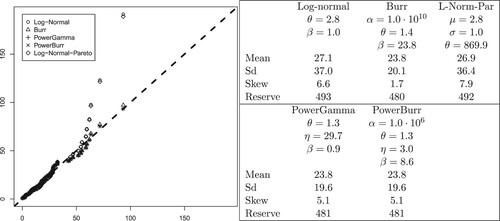
5. Example: automobile insurance

The example is taken from Bølviken (2014) and consists of n = 6446 claims of cost due to personal injuries in motor insurance with the deductible subtracted. This means that the claims are left-truncated at the deductible, but since the deductible is subtracted, the distribution still starts at 0, and we may use the distributions from Section 4 without modifications. The claims include cost due to personal injuries and are heavy-tailed with skewness 5.6 and kurtosis 71.2. The data are around 25 years old with mean and standard deviation 23.9 and 28.9 (in Norwegian kroner, NOK, about ten in one EUR) which would have been higher today. Among the five two-parameter distributions considered in this paper, the log-Normal was the only one providing a reasonable fit to the data, as judged from a Q-Q-plot, though it does not quite capture the largest claims. Its parameters are shown in the right panel of Figure 1, along with the mean, the standard deviation and the skewness. We also estimated the $99\mathrm{\%}$ reserve, assuming a Poisson distributed claim number with $\lambda =10$ expected incidents, based on ten million simulations This is shown in the same table, and so are corresponding results for the Burr, the PowerGamma and the PowerBurr families. As in the simulations of Section 4, we included the log-Normal-Pareto mixture as a reference. The results from the different distributions are quite similar, except for the skewness. The discrepancy between the smallest and largest projection of the reserve is no more than $2.5\mathrm{\%}$.

Figure 1. Five families of distributions fitted the automobile data with Q-Q-plots on the left and parameter estimates and statistical summary on the right.

Q-Q-plots of the five fitted distributions are shown in the left panel of Figure 1. They suggest that all five distributions fit the automobile insurance data reasonably well, except for the PowerGamma and also the log-Normal far out in the tail. The downward curvatures corresponds to an underestimation of the risk. This is reflected in a lower skewness than for the other families of distributions, and for the PowerGamma also a lower standard deviation. In this case, a Pareto element in the multi-parameter modeling, capturing the heavy tail of the data, seems required for a good fit. This is provided by both the Burr and the PowerBurr distributions, as they both have the Pareto distribution as a special case. For the same reason, the log-Normal-Pareto also gives a better fit to the data than the log-Normal in the tail.

As the Norwegian car insurance dataset is quite large, we also wanted to try the fit to a much smaller one. Therefore, we drew a random sub-sample of 64 claims from automobile insurance data, corresponding to 1/100 of its size. The resulting sample had a mean of 23.8, a standard deviation of 19.7 and a skewness of 1.3. We fitted the same five distributions as to the original data, and the corresponding results are shown in Figure 2. The Burr, PowerGamma and PowerBurr all provide a rather good fit to the data, also in the tail, as seen from the Q-Q-plot to the left. The fitted log-Normal is now much too heavy-tailed, which is also reflected in the corresponding standard deviation. In this case, the fitted log-Normal-Pareto mixture is essentially the same as the log-Normal, with the same parameters for the log-Normal part and a very high threshold parameter, and therefore does not fit the data particularly well.

Figure 2. Five families of distributions fitted to a random sample of 64 observations from the automobile data with Q-Q-plots on the left and parameter estimates and statistical summary on the right.

6. Concluding remarks

The Box-Cox transformed Gamma and Burr variables lead to models with many of the usual two- parameter families included as special cases, exactly or approximately. If the true distribution is on the boundary of the parameter space, as in the case of the log-normal, the best fit may involve very large (or small) parameters, but there is nothing wrong in using the computer solution as it is even if it could have been interpreted as some simpler sub-model. This is the convenient way of programming a completely automatized procedure with the computer converting loss data to actuarial evaluations on its own.

In unimodal families fitted distributions are much more stable than parameter estimates, and over-parameterization did not raise errors in actuarial projections substantially unless the parent distribution was very heavy-tailed. This was demonstrated by Monte Carlo and also by asymptotics as the number of historical losses $n\to \mathrm{\infty }$. Much of the latter argument used the log-normal as a vehicle, and its special properties allowed us to derive simple mathematical expressions for asymptotic errors, in particular prove that they are the same under PowerGamma and PowerBurr.

Acknowledgments

The authors wish to thank the two Reviewers and the Associate Editor for their helpful and constructive comments and suggestions.

Disclosure statement

No potential conflict of interest was reported by the author(s).

Appendices

Appendix 1.

Burr uncertainty for Pareto data

Section 3.2 required the information matrix for the Burr family and the gradient vectors for its moments and percentiles. If $I^{\text{bu}}$ is the information matrix with elements $I_{\mathrm{\alpha \alpha }}^{\text{bu}}$, $I_{\mathrm{\alpha \theta }}^{\text{bu}}$ and so on, then $\begin{array}{rl}& I_{\mathrm{\alpha \alpha }}^{\mathrm{bu}}={\psi }_1\left(\alpha \right)-{\psi }_1(\theta +\alpha )-\frac{\theta }{\alpha }{h}_{\mathrm{\alpha \theta }}^{\mathrm{bu}},I_{\mathrm{\alpha \theta }}^{\mathrm{bu}}=-{\psi }_1(\theta +\alpha )+h_{\mathrm{\alpha \theta }},I_{\alpha \text{β}}^{\mathrm{bu}}=-\frac{\theta }{(\theta +\alpha )(\theta +\alpha +1)}{\text{β}}^{-1},\\ & I_{\mathrm{\theta \theta }}^{\mathrm{bu}}={\psi }_1\left(\theta \right)-{\psi }_1(\theta +\alpha )-\frac{\alpha }{\theta }{h}_{\mathrm{\alpha \theta }},I_{\theta \text{β}}^{\mathrm{bu}}=\frac{\alpha }{(\theta +\alpha )(\theta +\alpha +1)}{\text{β}}^{-1},\\ & I_{\text{ββ}}^{\mathrm{bu}}=\frac{\mathrm{\theta \alpha }}{\theta +\alpha +1}{\text{β}}^{-2}\end{array}$where ${\psi }_1\left(z\right)=\frac{d^2\log \left\{\mathrm{\Gamma }\right(z\left)\right\}}{\mathrm{d}{z}^2}\text{and}{h}_{\mathrm{\alpha \theta }}=\frac{\theta +\alpha +2}{(\theta +\alpha )(\theta +\alpha +1)}.$The derivation of $I^{\text{bu}}$ from the density function (9(9) $I_{\mathrm{ij}}=E\left(\frac{\mathrm{\partial }\log \left\{f\right(Z;\mathit{p})}{\mathrm{\partial }{p}_i}\frac{\mathrm{\partial }\log \left\{f\right(Z;\mathit{p})}{\mathrm{\partial }{p}_j}\right),v_{\mathrm{ki}}=\frac{\mathrm{\partial }{\mu }_k\left(\mathbf{p}\right)}{\mathrm{\partial }{p}_i}\text{and}{v}_{\mathrm{ϵi}}=\frac{\mathrm{\partial }{q}_{ϵ}\left(\mathbf{p}\right)}{\mathrm{\partial }{p}_i},i,j=1,\dots ,d.$(9) ) is straightforward (albeit lengthy) and is omitted.

The gradient vectors for moments and percentiles are most conveniently calculated by differentiating their expressions numerically. The k'th order moment was given in (3(3) $E\left(Z^k\right)={\left(\frac{\alpha }{\theta }\right)}^k\left(\prod _{j=1}^k\frac{\theta +j-1}{\alpha -j}\right){\text{β}}^k,k=1,2,\dots$(3) ) whereas for the percentiles there is a simple relationship between Burr and Beta variables that can be utilized. Let $b_{\mathrm{ϵ\alpha \theta }}$ be the ϵ-percentile of the Beta distribution with shape parameters α and θ, available in standard software. Then $\alpha (b_{\mathrm{ϵ\alpha \theta }}^{-1}-1)\text{β}/\theta$ is the same Burr percentile.

Appendix 2.

Asymptotics in tilting models

A.1. General

Several of the uncertainty evaluations in Section 3 apply to models with density functions of the form (A1) $f(z;\nu ,\mathit{p})=f(z;\mathit{p}){\mathrm{e}}^{a(z;\mathit{p})\nu +o\left(\nu \right)}$(A1) with ν a tilting parameter adding to the parameter vector $\mathit{p}$ and with $a(z;\mathit{p})$ a known function. Note that ν is a transformation of those in Section 3, but when using likelihoods this does not affect uncertainty. The idea is to study how much the asymptotic standard deviation of moments and percentile estimates go up when we fit $f(z;\nu ,\mathit{p})$ for data generated by its limit $f(z;\mathit{p})$ as $\nu \to 0$. This requires the information matrix $I^{\nu }$ under $f(z;\nu ,\mathit{p})$ and the gradient vector ${\mathit{v}}^{\nu }$ of the quantity $\psi =\psi (\nu ,\mathit{p})$ of interest, again in the limit as $\nu \to 0$. Notation with superscript ν, for example $E^{\nu }$ and $q_{ϵ}^{\nu }$ for expectation and ϵ-percentile, applies to $f(z;\nu ,\mathit{p})$ whereas E and $q_{ϵ}$ without ν refer to $f(z;\mathit{p})$.

The information matrix $I^{\nu }$ and gradient vector ${\mathit{v}}^{\nu }$ under $f(z;\nu ,\mathit{p})$ are of the form (A2) $I^{\nu }=\left(\begin{array}{cc}{I}_{\mathrm{\nu \nu }}^{\nu }& I_{\nu \mathit{p}}^{\nu }\\ I_{\mathit{p}\nu }^{\nu }& I_{\mathit{pp}}^{\nu }\end{array}\right)\text{and}{v}^{\nu }=(v_{\nu }^{\nu },{\mathit{v}}_{\mathit{p}}^{\nu })$(A2) with $I_{\nu \mathit{p}}^{\nu }$ and $v_{\mathit{p}}^{\nu }$ row vectors. A recepy for calculating the limits of these quantities is (A3) $\begin{array}{rl}& \underset{\nu \to 0}{lim}{I}_{\mathit{pp}}^{\nu }=I_{\mathit{pp}}\text{and}\underset{\nu \to 0}{lim}{v}_{\mathit{p}}^{\nu }=v_{\mathit{p}},\end{array}$(A3) (A4) $\begin{array}{rl}& \underset{\nu \to 0}{lim}{I}_{\mathrm{\nu \nu }}^{\nu }=E\left\{a\right(Z;\mathit{p}){\}}^2\text{and}\underset{\nu \to 0}{lim}{I}_{\nu \mathit{p}}^{\nu }=E\left(a\right(Z;\mathit{p}\left)\frac{\mathrm{\partial }\log \left\{f\right(Z;\mathit{p}\left)\right\}}{\mathrm{\partial }\mathit{p}}\right),\end{array}$(A4) (A5) $\begin{array}{rl}& \underset{\nu \to 0}{lim}{v}_{\nu }^{\nu }=E\left\{a\right(Z;\mathit{p}\left)Z^k\right\}\text{if}\psi =E^{\nu }\left(Z^k\right),\end{array}$(A5) (A6) $\begin{array}{rl}& \underset{\nu \to 0}{lim}{v}_{\nu }^{\nu }=-\frac{{\int }_0^{q_{ϵ}}a(z;\mathit{p})f(z;\mathit{p})\mathrm{d}z}{f(q_{ϵ};\mathit{p})}\text{if}\psi =q_{ϵ}^{\nu }.\end{array}$(A6) To verify this start by recalling that $I_{\mathit{pp}}$ and ${\mathit{v}}_{\mathit{p}}$ in (A3(A3) $\begin{array}{rl}& \underset{\nu \to 0}{lim}{I}_{\mathit{pp}}^{\nu }=I_{\mathit{pp}}\text{and}\underset{\nu \to 0}{lim}{v}_{\mathit{p}}^{\nu }=v_{\mathit{p}},\end{array}$(A3) ) are information matrix and gradient vector under $f(z;\mathit{p})$, and become the limits as stated since $f(z;\nu ,\mathit{p})\to f(z;\mathit{p})$ when $\nu \to 0$. Next note that $I_{\mathrm{\nu \nu }}^{\nu }=E^{\nu }{\left(\frac{\mathrm{\partial }\log \left\{f\right(z;\nu ,\mathit{p}\left)\right\}}{\mathrm{\partial }\nu }\right)}^2\text{and}{I}_{\nu \mathit{p}}^{\nu }=E^{\nu }\left(\frac{\mathrm{\partial }\log \left\{f\right(z;\nu ,\mathit{p}\left)\right\}}{\mathrm{\partial }\nu }\frac{\mathrm{\partial }\log \left\{f\right(z;\nu ,\mathit{p}\left)\right\}}{\mathrm{\partial }\mathit{p}}\right),$and inserting (A1(A1) $f(z;\nu ,\mathit{p})=f(z;\mathit{p}){\mathrm{e}}^{a(z;\mathit{p})\nu +o\left(\nu \right)}$(A1) ) implies (A4(A4) $\begin{array}{rl}& \underset{\nu \to 0}{lim}{I}_{\mathrm{\nu \nu }}^{\nu }=E\left\{a\right(Z;\mathit{p}){\}}^2\text{and}\underset{\nu \to 0}{lim}{I}_{\nu \mathit{p}}^{\nu }=E\left(a\right(Z;\mathit{p}\left)\frac{\mathrm{\partial }\log \left\{f\right(Z;\mathit{p}\left)\right\}}{\mathrm{\partial }\mathit{p}}\right),\end{array}$(A4) ). The limits for the gradients remain. The k'th order moment is $E^{\nu }\left(Z^k\right)={\int }_0^{\mathrm{\infty }}{z}^{k}f(z;\nu ,\mathit{p})\mathrm{d}z,$and replacing the density function by (A1(A1) $f(z;\nu ,\mathit{p})=f(z;\mathit{p}){\mathrm{e}}^{a(z;\mathit{p})\nu +o\left(\nu \right)}$(A1) ) and then differentiating leads to (A5(A5) $\begin{array}{rl}& \underset{\nu \to 0}{lim}{v}_{\nu }^{\nu }=E\left\{a\right(Z;\mathit{p}\left)Z^k\right\}\text{if}\psi =E^{\nu }\left(Z^k\right),\end{array}$(A5) ). Finally, the ϵ-percentile $q_{ϵ}^{\nu }$ is from (A1(A1) $f(z;\nu ,\mathit{p})=f(z;\mathit{p}){\mathrm{e}}^{a(z;\mathit{p})\nu +o\left(\nu \right)}$(A1) ) the solution of ${\int }_0^{q_{ϵ}^{\nu }}f(z;\mathit{p}){\mathrm{e}}^{a(z;\mathit{p})\nu +o\left(\nu \right)}\mathrm{d}z=ϵ$which when differentiated with respect to ν yields $f(q_{ϵ}^{\nu };\mathit{p})\frac{\mathrm{\partial }{q}_{ϵ}^{\nu }}{\mathrm{\partial }\nu }+{\int }_0^{q_{ϵ}^{\nu }}f(z;\mathit{p})a(z;\mathit{p})\mathrm{d}z+o\left(1\right)=0$and (A6(A6) $\begin{array}{rl}& \underset{\nu \to 0}{lim}{v}_{\nu }^{\nu }=-\frac{{\int }_0^{q_{ϵ}}a(z;\mathit{p})f(z;\mathit{p})\mathrm{d}z}{f(q_{ϵ};\mathit{p})}\text{if}\psi =q_{ϵ}^{\nu }.\end{array}$(A6) ) follows since $q_{ϵ}^{\nu }\to q_{ϵ}$.

A.2. Burr uncertainty for Gamma data

The asymptotics when the Burr model is fitted Gamma data is covered by Section A.1. Start with the expression for the Burr density function in (2(2) $f\left(x\right)=\frac{\mathrm{\Gamma }(\alpha +\theta )}{\mathrm{\Gamma }\left(\alpha \right)\mathrm{\Gamma }\left(\theta \right)}{\left(\frac{\alpha }{\theta }\right)}^{\alpha }\frac{x^{\theta -1}}{(\alpha /\theta +x{)}^{\alpha +\theta }},x>0.$(2) ). It applies when $\text{β}=1$, but when it is rewritten for general β and with $\nu =1/\alpha$ replacing α, it becomes $f^{\mathrm{bu}}(z;\nu ,\theta ,\text{β})=\frac{\mathrm{\Gamma }({\nu }^{-1}+\theta )}{\mathrm{\Gamma }\left({\nu }^{-1}\right)\mathrm{\Gamma }\left(\theta \right)}\frac{(\mathrm{\nu \theta }{)}^{\theta }}{\text{β}}\frac{(z/\text{β}{)}^{\theta -1}}{(1+\mathrm{\nu \theta z}/\text{β}{)}^{{\nu }^{-1}+\theta }}.$Its limit when $\alpha \to \mathrm{\infty }$ or equivalently $\nu \to 0$ is the Gamma density function $f^{\mathrm{ga}}(z;\theta ,\text{β})=\frac{{\theta }^{\theta }}{\mathrm{\Gamma }\left(\theta \right)}\frac{1}{\text{β}}(z/\text{β}{)}^{\theta -1}{\mathrm{e}}^{-\mathrm{\theta z}/\text{β}},$and it is shown below that $f^{\text{bu}}(z;\nu ,\theta ,\text{β})$ and $f^{\text{ga}}(z;\theta ,\text{β})$ are connected by the tilting relationship (A1(A1) $f(z;\nu ,\mathit{p})=f(z;\mathit{p}){\mathrm{e}}^{a(z;\mathit{p})\nu +o\left(\nu \right)}$(A1) ) with (A7) $a(z;\theta ,\text{β})=\frac{1}{2}{\theta }^2{\left(\frac{z}{\text{β}}\right)}^2-{\theta }^2\frac{z}{\text{β}}+\frac{1}{2}({\theta }^2-\theta )$(A7) Table 3 was computed by inserting this function into (A3(A3) $\begin{array}{rl}& \underset{\nu \to 0}{lim}{I}_{\mathit{pp}}^{\nu }=I_{\mathit{pp}}\text{and}\underset{\nu \to 0}{lim}{v}_{\mathit{p}}^{\nu }=v_{\mathit{p}},\end{array}$(A3) )–(A6(A6) $\begin{array}{rl}& \underset{\nu \to 0}{lim}{v}_{\nu }^{\nu }=-\frac{{\int }_0^{q_{ϵ}}a(z;\mathit{p})f(z;\mathit{p})\mathrm{d}z}{f(q_{ϵ};\mathit{p})}\text{if}\psi =q_{ϵ}^{\nu }.\end{array}$(A6) ). Calculations were numerical since simple mathematical expressions are not available.

To verify (A7(A7) $a(z;\theta ,\text{β})=\frac{1}{2}{\theta }^2{\left(\frac{z}{\text{β}}\right)}^2-{\theta }^2\frac{z}{\text{β}}+\frac{1}{2}({\theta }^2-\theta )$(A7) ) note that the logarithm of the ratio between $f^{\text{bu}}(z;\nu ,\theta ,\text{β})$ and $f^{\text{ga}}(z;\theta ,\text{β})$ is $\log \left(\frac{f^{\mathrm{bu}}(z;\nu ,\theta ,\text{β})}{f^{\mathrm{ga}}(z;\theta ,\text{β})}\right)=\log \left\{\mathrm{\Gamma }\right({\nu }^{-1}+\theta \left)\right\}-\log \left\{\mathrm{\Gamma }\right({\nu }^{-1}\}+\mathrm{\theta log}(\nu )-({\nu }^{-1}+\theta )\log (1+\mathrm{\nu \theta z}/\text{β})+\mathrm{\theta z}/\text{β}.$The two log-Gamma functions can be simplified though the tail approximation (A8) $\log \left\{\mathrm{\Gamma }\right(z\left)\right\}=(z-1/2)\log \left(z\right)-z+\log \left(\sqrt{2\pi }\right)+o\left(z^{-1/2}\right)$(A8) whereas the Taylor series for $\log (1+z)$ yields $\log (1+\mathrm{\nu \theta z}/\text{β})=\mathrm{\nu \theta z}/\text{β}-\frac{1}{2}(\mathrm{\nu \theta z}/\text{β}{)}^2+o({\nu }^2),$and after some simple calculations $\log \left(\frac{f^{\mathrm{bu}}(z;\nu ,\theta ,\text{β})}{f^{\mathrm{ga}}(z;\theta ,\text{β})}\right)=\mathrm{\nu a}(z;\theta ,\text{β})+o\left(\nu \right)$with $a(z;\theta ,\text{β})$ as in (A7(A7) $a(z;\theta ,\text{β})=\frac{1}{2}{\theta }^2{\left(\frac{z}{\text{β}}\right)}^2-{\theta }^2\frac{z}{\text{β}}+\frac{1}{2}({\theta }^2-\theta )$(A7) ).

Appendix 3.

PowerGamma asymptotics

A.3. Tilting against the log-normal

The PowerGamma variable $Z=\text{β}\{1+G_{\theta }{)}^{\eta }-1\}$ has the density function (A9) $f^{\mathrm{pg}}(z;\theta ,\eta ,\text{β})=\frac{{\theta }^{\theta }}{\mathrm{\Gamma }\left(\theta \right)}\frac{1}{\text{β}\eta }{x}^{\theta -1}{\mathrm{e}}^{-\mathrm{\theta x}}(1+x{)}^{1-\eta }\text{where}x=(1+z/\text{β}{)}^{1/\eta }-1.$(A9) It was claimed in Section 3.3 that it can under a suitable reparameterization be tilted against a log-normal density function as $\theta \to \mathrm{\infty }$. Introduce new parameters $\nu =1/\sqrt{\theta },\text{β}=\xi {\mathrm{e}}^{-\log \left(4\right)\sigma /\nu },\eta =2\sigma /\nu$so that limits are in terms of $\nu \to 0$. With the new parameters the density function in (A9(A9) $f^{\mathrm{pg}}(z;\theta ,\eta ,\text{β})=\frac{{\theta }^{\theta }}{\mathrm{\Gamma }\left(\theta \right)}\frac{1}{\text{β}\eta }{x}^{\theta -1}{\mathrm{e}}^{-\mathrm{\theta x}}(1+x{)}^{1-\eta }\text{where}x=(1+z/\text{β}{)}^{1/\eta }-1.$(A9) ) is on log-form (A10) $\log \left\{f^{\mathrm{pg}}\right(z;\nu ,\xi ,\sigma \left)\right\}=c_{\nu }+({\nu }^{-2}-1)\log \left(x\right)-{\nu }^{-2}x+(1-2\sigma /\nu )\log (1+x)$(A10) where $c_{\nu }=-2{\nu }^{-2}\log \left(\nu \right)-\log \left\{\mathrm{\Gamma }\right({\nu }^{-2}\left)\right\}+\log \left(4\right)\sigma {\nu }^{-1}+\log \left(\nu \right)-\log \left(2\mathrm{\sigma \xi }\right).$By invoking the tail series (A8(A8) $\log \left\{\mathrm{\Gamma }\right(z\left)\right\}=(z-1/2)\log \left(z\right)-z+\log \left(\sqrt{2\pi }\right)+o\left(z^{-1/2}\right)$(A8) ) for the log Gamma function $c_{\nu }$ reduces to (A11) $c_{\nu }={\nu }^{-2}+\log \left(4\right)\sigma {\nu }^{-1}-\log \left(\sqrt{8\pi }\mathrm{\sigma \xi }\right)+o\left(\nu \right).$(A11) To simplify the other terms in (A10(A10) $\log \left\{f^{\mathrm{pg}}\right(z;\nu ,\xi ,\sigma \left)\right\}=c_{\nu }+({\nu }^{-2}-1)\log \left(x\right)-{\nu }^{-2}x+(1-2\sigma /\nu )\log (1+x)$(A10) ) start by noting that (A9(A9) $f^{\mathrm{pg}}(z;\theta ,\eta ,\text{β})=\frac{{\theta }^{\theta }}{\mathrm{\Gamma }\left(\theta \right)}\frac{1}{\text{β}\eta }{x}^{\theta -1}{\mathrm{e}}^{-\mathrm{\theta x}}(1+x{)}^{1-\eta }\text{where}x=(1+z/\text{β}{)}^{1/\eta }-1.$(A9) ) right yields $\log (1+x)=\log (1+z/\text{β})/\eta =\log \left(z/\text{β}\right)/\eta +\log (1+\text{β}/z)/\eta$where the second term on the right through β tends to 0 at exponential rate as $\nu \to 0$. Hence after inserting for η and β (A12) $\log (1+x)=\log \left(2\right)+\frac{y}{2}\nu +o\left({\nu }^3\right)\text{where}y=\log \left(z/\xi \right)/\sigma .$(A12) This will be the vehicle for much of the calculations to follow. Utilize that $x={\mathrm{e}}^{\log (1+x)}-1=2{\mathrm{e}}^{\left(y/2\right)\nu +o\left({\nu }^3\right)}-1$which from the Taylor series of the exponential function becomes (A13) $x=1+\mathrm{y\nu }+\frac{y^2}{4}{\nu }^2+\frac{y^3}{24}{\nu }^3+o\left({\nu }^3\right).$(A13) Take logarithms on both sides and use the Taylor series of the logarithmic function. Some straightforward calculations and rearrangements then lead to (A14) $\log \left(x\right)=\mathrm{y\nu }-\frac{y^2}{4}{\nu }^2+\frac{y^3}{8}{\nu }^3+o\left({\nu }^3\right)$(A14) Finally, when inserting (A11(A11) $c_{\nu }={\nu }^{-2}+\log \left(4\right)\sigma {\nu }^{-1}-\log \left(\sqrt{8\pi }\mathrm{\sigma \xi }\right)+o\left(\nu \right).$(A11) )–(A14(A14) $\log \left(x\right)=\mathrm{y\nu }-\frac{y^2}{4}{\nu }^2+\frac{y^3}{8}{\nu }^3+o\left({\nu }^3\right)$(A14) ) into (A10(A10) $\log \left\{f^{\mathrm{pg}}\right(z;\nu ,\xi ,\sigma \left)\right\}=c_{\nu }+({\nu }^{-2}-1)\log \left(x\right)-{\nu }^{-2}x+(1-2\sigma /\nu )\log (1+x)$(A10) ), a lot of terms cancel, and it follows after some straightforward manipulations that $\log \left\{f^{\mathrm{pg}}\right(z;\nu ,\xi ,\sigma \left)\right\}=-\log \left(\sqrt{2\pi }\mathrm{\sigma \xi }\right)-\mathrm{\sigma y}-\frac{1}{2}{y}^2+(-\frac{y}{2}+\frac{y^3}{12})\nu +o\left(\nu \right)$or $\log \left\{f^{\mathrm{pg}}\right(z;\nu ,\xi ,\sigma \left)\right\}=\log \left\{f^{\ln }\right(z;\xi ,\sigma \left)\right\}+(-\frac{\log \left(z/\xi \right)}{2\sigma }+\frac{{\log }^3\left(z/\xi \right)}{12{\sigma }^3})\nu +o\left(\nu \right)$after inserting $y=\log \left(z/\xi \right)/\sigma$. This is the tilting relation (15(15) $f^{\mathrm{pg}}(z;\theta ,\xi ,\sigma )=f^{\ln }(z;\xi ,\sigma ){\mathrm{e}}^{a(z;\xi ,\sigma ){\theta }^{-1/2}+o\left({\theta }^{-1/2}\right)},a(z;\xi ,\sigma )=-\frac{\log \left(z/\xi \right)}{2\sigma }+\frac{{\log }^3\left(z/\xi \right)}{12{\sigma }^3}.$(15) ).

A.4. The information matrix

The information matrix when the PowerGamma family is fitted log-normal data is (A15) $\underset{\nu \to 0}{lim}{I}^{\mathrm{pg}}=\left(\begin{array}{ccc}5/48& -1/\left(4\mathrm{\xi \sigma }\right)& 0\\ -1/\left(4\mathrm{\xi \sigma }\right)& 1/\left({\xi }^2{\sigma }^2\right)& 0\\ 0& 0& 2/{\sigma }^2\end{array}\right)$(A15) To verify this start by noting that when Z is log-normal, then $Y=\log \left(Z/\xi \right)/\sigma$ is $N(0,1)$ with second, fourth and sixth order moments 1, 3 and 15. Hence (A4(A4) $\begin{array}{rl}& \underset{\nu \to 0}{lim}{I}_{\mathrm{\nu \nu }}^{\nu }=E\left\{a\right(Z;\mathit{p}){\}}^2\text{and}\underset{\nu \to 0}{lim}{I}_{\nu \mathit{p}}^{\nu }=E\left(a\right(Z;\mathit{p}\left)\frac{\mathrm{\partial }\log \left\{f\right(Z;\mathit{p}\left)\right\}}{\mathrm{\partial }\mathit{p}}\right),\end{array}$(A4) ) left and (15(15) $f^{\mathrm{pg}}(z;\theta ,\xi ,\sigma )=f^{\ln }(z;\xi ,\sigma ){\mathrm{e}}^{a(z;\xi ,\sigma ){\theta }^{-1/2}+o\left({\theta }^{-1/2}\right)},a(z;\xi ,\sigma )=-\frac{\log \left(z/\xi \right)}{2\sigma }+\frac{{\log }^3\left(z/\xi \right)}{12{\sigma }^3}.$(15) ) right yield $\underset{\nu \to 0}{lim}{I}_{\mathrm{\nu \nu }}^{\mathrm{pg}}=E{(-\frac{Y}{2}+\frac{Y^3}{12})}^2=E(\frac{Y^2}{4}-\frac{Y^4}{12}+\frac{Y^6}{144})=\frac{5}{48}.$Next from (14(14) $f^{\ln }(z;\xi ,\sigma )=\frac{1}{\sqrt{2\pi }\sigma }{z}^{-1}{\mathrm{e}}^{-{\log }^2\left(z/\xi \right)/\left(2{\sigma }^2\right)}$(14) ) $\frac{\mathrm{\partial }\log \left\{f^{\ln }\right(Z;\xi ,\sigma \left)\right\}}{\mathrm{\partial }\xi }=\frac{\log \left(Z/\xi \right)}{\sigma }\frac{1}{\mathrm{\xi \sigma }}=\frac{Y}{\mathrm{\xi \sigma }},\frac{\mathrm{\partial }\log \left\{f^{\ln }\right(Z;\xi ,\sigma \left)\right\}}{\mathrm{\partial }\sigma }=(\frac{{\log }^2\left(Z/\xi \right)}{{\sigma }^2}-1)\frac{1}{\sigma }=\frac{Y^2-1}{\sigma }$so that by (A4(A4) $\begin{array}{rl}& \underset{\nu \to 0}{lim}{I}_{\mathrm{\nu \nu }}^{\nu }=E\left\{a\right(Z;\mathit{p}){\}}^2\text{and}\underset{\nu \to 0}{lim}{I}_{\nu \mathit{p}}^{\nu }=E\left(a\right(Z;\mathit{p}\left)\frac{\mathrm{\partial }\log \left\{f\right(Z;\mathit{p}\left)\right\}}{\mathrm{\partial }\mathit{p}}\right),\end{array}$(A4) ) right $\underset{\nu \to 0}{lim}{I}_{\mathrm{\nu \xi }}^{\mathrm{pg}}=E(-\frac{Y}{2}+\frac{Y^3}{12})\frac{Y}{\mathrm{\xi \sigma }}=-\frac{1}{4\mathrm{\xi \sigma }},\underset{\nu \to 0}{lim}{I}_{\mathrm{\nu \xi }}^{\mathrm{pg}}=E(-\frac{Y}{2}+\frac{Y^3}{12})\frac{Y^2-1}{\sigma }=0$where the right hand side vanishes in expectation since all powers of Y are odd when multiplied out. This establishes the first row and column in (A15(A15) $\underset{\nu \to 0}{lim}{I}^{\mathrm{pg}}=\left(\begin{array}{ccc}5/48& -1/\left(4\mathrm{\xi \sigma }\right)& 0\\ -1/\left(4\mathrm{\xi \sigma }\right)& 1/\left({\xi }^2{\sigma }^2\right)& 0\\ 0& 0& 2/{\sigma }^2\end{array}\right)$(A15) ), and the rest are elementary results for the log-normal.

A.5. Moment estimation

The moment of order k under the log-normal is (A16) ${\mu }_k={\xi }^k{\mathrm{e}}^{k^2{\sigma }^2/2},$(A16) and we seek the asymptotic standard deviation of its estimate when the PowerGamma model has been fitted. We need the inverse of the matrix (A15(A15) $\underset{\nu \to 0}{lim}{I}^{\mathrm{pg}}=\left(\begin{array}{ccc}5/48& -1/\left(4\mathrm{\xi \sigma }\right)& 0\\ -1/\left(4\mathrm{\xi \sigma }\right)& 1/\left({\xi }^2{\sigma }^2\right)& 0\\ 0& 0& 2/{\sigma }^2\end{array}\right)$(A15) ) which is (A17) $\underset{\nu \to 0}{lim}(I^{\mathrm{pg}}{)}^{-1}=\left(\begin{array}{ccc}24& 6\mathrm{\xi \sigma }& 0\\ 6\mathrm{\xi \sigma }& 5{\sigma }^2{\xi }^2/2& 0\\ 0& 0& {\sigma }^2/2\end{array}\right)$(A17) and also the limit of the gradient ${\mathit{v}}^{\text{pg}}=(v_{\nu }^{\text{pg}},v_{\xi }^{\text{pg}},v_{\sigma }^{\text{pg}}{)}^T$. The latter is (A18) $\underset{\nu \to 0}{lim}{v}_{\nu }^{\mathrm{pg}}=(-\frac{\mathrm{k\sigma }}{4}+\frac{k^3{\sigma }^3}{12}){\mu }_k,\underset{\nu \to 0}{lim}{v}_{\xi }^{\mathrm{pg}}=\frac{k}{\xi }{\mu }_k,\underset{\nu \to 0}{lim}{v}_{\sigma }^{\mathrm{pg}}=k^2\sigma {\mu }_k$(A18) The limits for $v_{\xi }^{\text{pg}}$ and $v_{\sigma }^{\text{pg}}$ follows by differentiating (A16(A16) ${\mu }_k={\xi }^k{\mathrm{e}}^{k^2{\sigma }^2/2},$(A16) ) whereas the one for $v_{\nu }^{\text{pg}}$ is determined from (A5(A5) $\begin{array}{rl}& \underset{\nu \to 0}{lim}{v}_{\nu }^{\nu }=E\left\{a\right(Z;\mathit{p}\left)Z^k\right\}\text{if}\psi =E^{\nu }\left(Z^k\right),\end{array}$(A5) ) and (15(15) $f^{\mathrm{pg}}(z;\theta ,\xi ,\sigma )=f^{\ln }(z;\xi ,\sigma ){\mathrm{e}}^{a(z;\xi ,\sigma ){\theta }^{-1/2}+o\left({\theta }^{-1/2}\right)},a(z;\xi ,\sigma )=-\frac{\log \left(z/\xi \right)}{2\sigma }+\frac{{\log }^3\left(z/\xi \right)}{12{\sigma }^3}.$(15) ) right which yield $\underset{\nu \to 0}{lim}{v}_{\nu }^{\mathrm{pg}}=E\left(a\right(Z;\xi ,\sigma \left)Z^k\right)={\xi }^{k}E(-\frac{Y}{2}+\frac{Y^3}{12}){\mathrm{e}}^{\mathrm{k\sigma Y}},$and an elementary calculation utilizing that $Y\sim N(0,1)$ closes the argument.

Let $s_k^{\text{pg}}(\xi ,\sigma )/\sqrt{n}$ be the asymptotic standard deviation for the moment estimate when fitting the PowerGamma model to log-normal data. Then $s_k^{\text{pg}}(\xi ,\sigma )$ is the limit of the square root of ${\mathit{v}}^{\text{pg}}\left(I^{\text{pg}}{)}^{-1}\right({\mathit{v}}^{\text{pg}}{)}^T$ and becomes $s_k^{\mathrm{pg}}(\xi ,\sigma )={(k^2{\sigma }^2+\frac{k^4{\sigma }^4}{2}+\frac{k^6{\sigma }^6}{6})}^{1/2}{\mu }_k$which is to be compared with its counterpart $s_k^{\text{ln}}(\xi ,\sigma )$ under log-normal fitting. Now the information matrix is the $2\times 2$ block in the lower, left corner of (A15(A15) $\underset{\nu \to 0}{lim}{I}^{\mathrm{pg}}=\left(\begin{array}{ccc}5/48& -1/\left(4\mathrm{\xi \sigma }\right)& 0\\ -1/\left(4\mathrm{\xi \sigma }\right)& 1/\left({\xi }^2{\sigma }^2\right)& 0\\ 0& 0& 2/{\sigma }^2\end{array}\right)$(A15) ) and the gradient the last two elements in (A18(A18) $\underset{\nu \to 0}{lim}{v}_{\nu }^{\mathrm{pg}}=(-\frac{\mathrm{k\sigma }}{4}+\frac{k^3{\sigma }^3}{12}){\mu }_k,\underset{\nu \to 0}{lim}{v}_{\xi }^{\mathrm{pg}}=\frac{k}{\xi }{\mu }_k,\underset{\nu \to 0}{lim}{v}_{\sigma }^{\mathrm{pg}}=k^2\sigma {\mu }_k$(A18) ) so that $s_k^{\ln }(\xi ,\sigma )={(k^2{\sigma }^2+\frac{k^4{\sigma }^4}{2})}^{1/2}{\mu }_k.$Hence ${\left(\frac{s_k^{\mathrm{pg}}(\xi ,\sigma )}{s_k^{\ln }(\xi ,\sigma )}\right)}^2=1+\frac{k^4{\sigma }^4}{6+3k^2{\sigma }^2},$leading to (17(17) $D_k^{\mathrm{pg}|\ln }(\xi ,\sigma )={(1+\frac{k^4{\sigma }^4}{6+3k^2{\sigma }^2})}^{1/2}-1\text{and}{D}_{ϵ}^{\mathrm{pg}|\ln }(\xi ,\sigma )={(1+\frac{({\varphi }_{ϵ}^2-1{)}^2}{3{\varphi }_{ϵ}^2+6})}^{1/2}-1.$(17) ) left.

A.6. Percentile estimation

The quantity we are now trying to estimate is (A19) $q_{ϵ}=\xi {\mathrm{e}}^{\sigma {\varphi }_{ϵ}}$(A19) with ${\varphi }_{ϵ}$ the ϵ-percentile of the standard normal. The study of asymptotic uncertainty is the same as above except for the gradient which has become (A20) $\underset{\nu \to 0}{lim}{v}_{\nu }^{\mathrm{pg}}=\frac{1}{3}(-1+\frac{{\varphi }_{ϵ}^2}{4})\sigma q_{ϵ},\underset{\nu \to 0}{lim}{v}_{\xi }^{\mathrm{pg}}=\frac{1}{\xi }{q}_{ϵ}\underset{\nu \to 0}{lim}{v}_{\sigma }^{\mathrm{pg}}={\varphi }_{ϵ}{q}_{ϵ}.$(A20) Only the expression for $v_{\nu }^{\text{pg}}$ requires a calculation since the rest are obvious consequences of differentiating (A19(A19) $q_{ϵ}=\xi {\mathrm{e}}^{\sigma {\varphi }_{ϵ}}$(A19) ). By (A6(A6) $\begin{array}{rl}& \underset{\nu \to 0}{lim}{v}_{\nu }^{\nu }=-\frac{{\int }_0^{q_{ϵ}}a(z;\mathit{p})f(z;\mathit{p})\mathrm{d}z}{f(q_{ϵ};\mathit{p})}\text{if}\psi =q_{ϵ}^{\nu }.\end{array}$(A6) ) $\underset{\nu \to 0}{lim}{v}_{\nu }^{\mathrm{pg}}=-\frac{{\int }_0^{q_{ϵ}}{f}^{\ln }(z;\xi ,\sigma )a(z;\xi ,\sigma )\mathrm{d}z}{f^{\mathrm{pg}}(q_{ϵ};\xi ,\sigma )}$where $f^{\text{pg}}(z;\xi ,\sigma )$ is the log-normal density function above and $a(z;\xi ,\sigma )$ is the function (15(15) $f^{\mathrm{pg}}(z;\theta ,\xi ,\sigma )=f^{\ln }(z;\xi ,\sigma ){\mathrm{e}}^{a(z;\xi ,\sigma ){\theta }^{-1/2}+o\left({\theta }^{-1/2}\right)},a(z;\xi ,\sigma )=-\frac{\log \left(z/\xi \right)}{2\sigma }+\frac{{\log }^3\left(z/\xi \right)}{12{\sigma }^3}.$(15) ) right. The integral is evaluated by substituting $y=\log \left(z/\xi \right)/\sigma$. With $\phi \left(y\right)=(2\pi {)}^{-1/2}{\mathrm{e}}^{-y^2/2}$ this yields (A21) ${\int }_0^{q_{ϵ}}{f}^{\ln }(z;\xi ,\sigma )a(z;\xi ,\sigma )\mathrm{d}z={\int }_{-\mathrm{\infty }}^{{\varphi }_{ϵ}}(-y/2+y^3/12)\phi \left(y\right)\mathrm{dy}=\frac{1}{3}(1-\frac{{\varphi }_{ϵ}^2}{4})\phi \left({\varphi }_{ϵ}\right).$(A21) whereas $f^{\ln }(q_{ϵ};\xi ,\sigma )=\frac{\phi \left({\varphi }_{ϵ}\right)}{\sigma q_{ϵ}},$and (A20(A20) $\underset{\nu \to 0}{lim}{v}_{\nu }^{\mathrm{pg}}=\frac{1}{3}(-1+\frac{{\varphi }_{ϵ}^2}{4})\sigma q_{ϵ},\underset{\nu \to 0}{lim}{v}_{\xi }^{\mathrm{pg}}=\frac{1}{\xi }{q}_{ϵ}\underset{\nu \to 0}{lim}{v}_{\sigma }^{\mathrm{pg}}={\varphi }_{ϵ}{q}_{ϵ}.$(A20) ) left follows.

The quadratic form when combining the vector (A20(A20) $\underset{\nu \to 0}{lim}{v}_{\nu }^{\mathrm{pg}}=\frac{1}{3}(-1+\frac{{\varphi }_{ϵ}^2}{4})\sigma q_{ϵ},\underset{\nu \to 0}{lim}{v}_{\xi }^{\mathrm{pg}}=\frac{1}{\xi }{q}_{ϵ}\underset{\nu \to 0}{lim}{v}_{\sigma }^{\mathrm{pg}}={\varphi }_{ϵ}{q}_{ϵ}.$(A20) ) with the matrix (A17(A17) $\underset{\nu \to 0}{lim}(I^{\mathrm{pg}}{)}^{-1}=\left(\begin{array}{ccc}24& 6\mathrm{\xi \sigma }& 0\\ 6\mathrm{\xi \sigma }& 5{\sigma }^2{\xi }^2/2& 0\\ 0& 0& {\sigma }^2/2\end{array}\right)$(A17) ) yields the coefficient $s_{ϵ}^{\text{pg}}(\xi ,\sigma )$ as $s_{ϵ}^{\mathrm{pg}}(\xi ,\sigma )={(\frac{24}{9}{(-1+\frac{{\varphi }_{ϵ}^2}{4})}^2+4(-1+\frac{{\varphi }_{ϵ}^2}{4})+\frac{5}{2}+\frac{1}{2}{\varphi }_{ϵ}^2)}^{1/2}\sigma q_{ϵ}$whereas for the log-normal the similar quantity is $s_{ϵ}^{\ln }(\xi ,\sigma )={(1+\frac{{\varphi }_{ϵ}^2}{2})}^{1/2}\sigma q_{ϵ}$after using the last two elements in (A20(A20) $\underset{\nu \to 0}{lim}{v}_{\nu }^{\mathrm{pg}}=\frac{1}{3}(-1+\frac{{\varphi }_{ϵ}^2}{4})\sigma q_{ϵ},\underset{\nu \to 0}{lim}{v}_{\xi }^{\mathrm{pg}}=\frac{1}{\xi }{q}_{ϵ}\underset{\nu \to 0}{lim}{v}_{\sigma }^{\mathrm{pg}}={\varphi }_{ϵ}{q}_{ϵ}.$(A20) ) as the gradient vector and the lower $2\times 2$ block in (A15(A15) $\underset{\nu \to 0}{lim}{I}^{\mathrm{pg}}=\left(\begin{array}{ccc}5/48& -1/\left(4\mathrm{\xi \sigma }\right)& 0\\ -1/\left(4\mathrm{\xi \sigma }\right)& 1/\left({\xi }^2{\sigma }^2\right)& 0\\ 0& 0& 2/{\sigma }^2\end{array}\right)$(A15) ) as information matrix. It follows that $\left\{s_{ϵ}^{\mathrm{pg}}\right(\xi ,\sigma ){\}}^2-\{s_{ϵ}^{\ln }(\xi ,\sigma ){\}}^2=\frac{1}{6}({\varphi }_{ϵ}^2-1{)}^2{\sigma }^2{q}_{ϵ}^2$so that $\frac{s_{ϵ}^{\mathrm{pg}}(\xi ,\sigma )}{s_{ϵ}^{\ln }(\xi ,\sigma )}={(1+\frac{({\varphi }_{ϵ}^2-1{)}^2}{3{\varphi }_{ϵ}^2+6})}^{1/2}$as claimed in (17(17) $D_k^{\mathrm{pg}|\ln }(\xi ,\sigma )={(1+\frac{k^4{\sigma }^4}{6+3k^2{\sigma }^2})}^{1/2}-1\text{and}{D}_{ϵ}^{\mathrm{pg}|\ln }(\xi ,\sigma )={(1+\frac{({\varphi }_{ϵ}^2-1{)}^2}{3{\varphi }_{ϵ}^2+6})}^{1/2}-1.$(17) ) right.

Appendix 4.

PowerBurr density

The PowerBurr model defined in (5(5) $Z=\text{β}\left\{\right(1+G_{\theta }{)}^{\eta }-1\}\text{and}Z=\text{β}\{(1+X{)}^{\eta }-1\}$(5) ) right has density function (A22) $f^{\mathrm{pb}}(z;\theta ,\xi ,\sigma ,\alpha )=\frac{\mathrm{\Gamma }(\theta +\alpha )}{\mathrm{\Gamma }\left(\alpha \right)\mathrm{\Gamma }\left(\theta \right)}{\left(\frac{\theta }{\alpha }\right)}^{\theta }\frac{1}{\eta \text{β}}\frac{x^{\theta -1}(1+x{)}^{1-\eta }}{(1+\mathrm{\theta x}/\alpha {)}^{\alpha +\theta }},x=(1+z/\text{β}{)}^{1/\eta }-1.$(A22)

References

- Bakar S., Hamzah N., Maghsoudi M. & Nadarajah S. (2015). Modeling loss data using composite models. Insurance: Mathematics and Economics 61, 146–154.
- Beirlant J., Teugels J. & Vynckier P. (1996). Practical analysis of extreme values. Leuven University Press.
- Bølviken E. (2014). Computation and modelling in insurance and finance. Cambridge University Press.
- Box G. & Cox D. (1964). An analysis of transformations (with discussion). Journal of the Royal Statistical Society Series B 26, 231–252.
- Burr I. J. (1942). Cumulative frequency functions. Annals of Mathematical Statistics 13, 215–232.
- Chan J. S. K., Choy S. T. B., Makov U. R. & Landsman Z. (2018). Modelling insurance losses using contaminated, generalized beta type II distributions. ASTIN Bulletin 48(02), 871–904.
- Cooray K. & Ananda M. M. A. (2005). Modeling actuarial data with composite lognormal-Pareto model. Scandinavian Actuarial Journal 2005, 642–660.
- Cummins J. D., Dionne G., MacDonald J. B. & Pritchett B. M. (1990). Applications of the GB2 family of distributions in modeling insurance loss processes. Insurance: Mathematics and Economics 9(4), 257–272.
- Embrechts P., Klüppelberg C. & Mikosch T. (Modelling extremal events. Stochastic Modelling and Applied Probability.1997). Springer Verlag.
- Gui W., Huang R. & Lin X. S. (2021). Fitting multivariate Erlang mixtures to data: a roughness penality approach. Journal of Computational and Applied Mathematics 386, 113216.
- Hoeting J. A., Madigan D., Raftery A. E. & Volinsky C. T. (1999). Bayesian model averaging: a tutorial. Statistical Science 14(4), 382–401.
- Huber P. (1967). The behavior of maximum likelihood estimates under nonstandard conditions. In Proceedings of the Fifth Berkely Symposium in Mathematical Statistics and Probability. University of California Press.
- Kleiber C. & Kotz S. (2003). Statistical size distributions in economics and actuarial sciences. Wiley.
- Lee S. & Lin X. (2010). Modeling and evaluating insurance losses via mixtures of Erlang distributions. North American Actuarial Journal 14(1), 107–130.
- Marlin P. (1984). Fitting the log-normal distribution to loss data subject to multiple deductibles. The Journal of Risk and Insurance 51( 4), 687–701.
- Miljkovic T. & Grün B. (2016). Modeling loss data using mixtures of distributions. Insurance: Mathematics and Economics 70, 387–396.
- Omari C. O., Nyambura S. G. & Mwangi J. M. W. (2018). Modeling the frequency and severity of auto insurance claims using statistical distributions. Journal of Mathematical Finance 8(1), 137–160.
- Reynkens T., Verbelen R., Beirlant J. & Antonio K. (2017). Modelling censored losses using splicing: a global fit strategy with mixed Erlang and extreme value distributions. Insurance Mathematics & Economics 77, 65–77.
- Scollnik D. P. M. (2007). On composite lognormal-Pareto distributions. Scandinavian Actuarial Journal2007(1), 20–33.
- Scollnik D. P. M. & Sun C. (2012). Modelling with Weibull-Pareto models. North American Actuarial Journal 16(2), 260–272.
- Scott P. W. (1992). Multivariate density estimation: theory, practice and visualization. John Wiley & Sons.
- Venter C. (1985). Transformed Beta and Gamma distributions and aggregate losses. Casually Actuarial Society 70, 156–193.
- Verbelen R., Gong L., Antonio K., Badescu A. & Lin S. (2015). Fitting extremes of Erlangs to censored and truncated data using the EM algorithm. ASTIN Bulletin 45, 729–758.
- White H. (1982). Maximum likelihood estimation of misspecified models. Econometrica 50(1), 1–25.
- White H. (1994). Estimation, inference and specification analysis. Cambridge: Cambridge University Press.
- Zuanetti D. & Diniz C. (2006). A lognormal model for insurance claims data. REVSTAT – Statistical Journal 4, 131–142.