Estimating Tree Diameter at Breast Height (DBH) Using iPad Pro LiDAR Sensor in Boreal Forests

Abstract

Traditional Diameter at Breast Height (DBH) mensuration is labor-intensive and costly. This scoping study explored the possibility of using the Apple iPad Pro Light Detection And Ranging (LiDAR) sensor to estimate DBH. Three plots were scanned in a research plantation near Thunder Bay, Canada. Sites consisted of either Black Spruce (Picea mariana) or Red Pine (Pinus resinosa) planted with different initial densities. DBH was manually measured for validation. Point clouds were acquired for each plot using three scanning patterns; circular, figure-8, and transect. Single and five cross sections of 4 or 10 cm in thickness were extracted from each point cloud, centered at 1.3 m above the ground. Two circle fitting algorithms (Pratt, Taubin) and two ellipse fitting algorithms (Taubin, Szpak) were applied to the extracted cross-sections to estimate DBH. Scanning pattern and curve-fitting formula significantly impacted DBH estimate accuracy (p-value ≤ 0.001), while cross-section count and thickness did not. The circular scanning pattern with a single 4 cm cross-section and a combination of circle- and ellipse-fitting formulas was the most accurate DBH estimation method (RMSE = 1.1 cm; 6.17%).

RÉSUMÉ

Le diamètre à la hauteur de poitrine (DHP) est mesuré traditionnellement en utilisant des méthodes coûteuses et nécessitant une importante main-d’œuvre. Cette étude a exploré la possibilité d‘utiliser le capteur de détection et de télémétrie par ondes lumineuses (LiDAR) d‘Apple, iPad Pro, pour estimer le DHP. Trois parcelles ont été scannées dans une plantation de recherche près de Thunder Bay, Ontario, Canada. Les sites étaient constitués d‘épinettes noires (Picea mariana) ou de pins rouges (Pinus resinosa) plantés avec différentes densités. Le DHP a été mesuré manuellement pour validation. Des nuages de points ont été acquis pour chaque parcelle à l‘aide de trois méthodes de balayage; circulaire, figure-8 et transect. Une seule section et cinq sections transversales de 4 ou 10 cm d‘épaisseur ont été extraites de chaque nuage de points, centrées à 1.3 m au-dessus du sol. Deux algorithmes d‘ajustement circulaire (Pratt, Taubin) et deux algorithmes d‘ajustement d‘ellipse (Taubin, Szpak) ont été appliqués aux sections transversales extraites pour estimer le DHP. Le modèle de balayage et la formule d‘ajustement de courbe ont eu une incidence significative sur la précision de l‘estimation du DHP (p ≤ 0,001), tandis que le nombre de sections transversales et l‘épaisseur n’ont pas eu d’incidence significative. Le modèle de balayage circulaire avec une seule section transversale de 4 cm et une combinaison de formules d’ajustement basées sur le cercle et l‘ellipse était la méthode d‘estimation la plus précise du DHP (RMSE = 1.1 cm; 6.17%).

Introduction

Forest Resource Inventories (FRIs) form the basis for understanding and monitoring dynamic changes in forests (White et al. 2016). FRIs are also the foundational layer of information used in forest management planning (Bilyk et al. 2021). As forest management policies and legislation have developed, the scope and depth of information required in an FRI have increased (Bilyk et al. 2021). Hence, the enhanced version of the FRI requires a wide range of information, covering many aspects of a forest, such as basal area, stem location, tree heights, crown area, and height to direct live crown for trees, and other values such as soil horizons and their depths (OMNRF 2021). Additionally, fast and accurate forest inventories are increasingly necessary for effective forest management (Müller et al. 2020). Diameter at Breast Height (DBH) is one of the most frequently measured attributes for FRIs (Chiappini et al. 2022). It corresponds to the diameter of a tree stem at 1.3 m above the ground. DBH is measured manually using a diameter tape or calipers, but these methods are time-consuming and costly (Aijazi et al. 2017). In addition to DBH, FRIs measure or calculate (based on field measurements) many other variables, including site-specific soil, species, density, and volume data. In Ontario, this is done to determine the suitability of a site for harvest and to identify specific methods of harvesting and regeneration best-suited for the site (OMNRF 2015).

Since the advent of Light Detection and Ranging (LiDAR) technologies, numerous studies have investigated different methods of using LiDAR to measure forest parameters (Blanco et al. 2015; Côté et al. 2011; Lovell et al. 2003; Woods et al. 2011). Airborne Laser Scanning (ALS) from manned aircrafts and ALS from Unmanned Aerial Vehicles (UAVs) are recognized as more efficient than terrestrial systems in terms of time required to create dense point clouds (Brede et al. 2017). However, unlike terrestrial systems, ALS cannot provide below-canopy stem profiles with a high enough point density to allow estimation of DBH (Dassot et al. 2011; Hyyppä et al. 2020; Woods et al. 2011). UAV LiDAR addresses many of the problems with ALS by capturing a high density of points in a versatile, customizable platform that can be flown above or below canopy, albeit with lower point densities than most Terrestrial Laser Scanning (TLS) systems (Brede et al. 2017). Therefore, TLS may be best suited for estimating DBH. TLS was first used for forest inventory by Hopkinson et al. (2004), who accurately measured or derived stem location, tree heights, DBH, site density, and timber volume from point cloud data. Bauwens et al. (2016) used TLS to accurately estimate other forest inventory metrics, including basal area, gap fraction, and Leaf Area Index (LAI) and confirmed that it is more time efficient than manual measurements.

Tree stem cross-sections were first modeled by Pfeifer and Winterhalder (2004), who used free-form b-spline formulas with mean square error to fit irregular curves to point cloud data. Later, Hopkinson et al. (2004) estimated DBH with a least-squares regression cylinder fit, applied to a single three-dimensional cross-section of each stem 1.25–1.75m above ground. Pfeifer and Winterhalder (2004) and other more recent studies have suggested that point cloud data should be acquired from multiple perspectives and capture much of the tree stem for accurate cross-section modeling due to tree stems’ irregular, uneven shapes (Hunčaga et al. 2020; Wang et al. 2022). Recently, Liang et al. (2018) found in a benchmarking study that using multiple scans of a forest plot significantly improved the accuracy of forest metrics estimated from TLS data. Despite the high accuracy of DBH estimations derived from TLS reported in recent studies, several factors, including device costs, have prevented these systems from being widely integrated in forest inventories (Calders et al. 2020; Luetzenburg et al. 2021).

Since the advent of the first terrestrial LiDAR scanners, device weight and size have decreased while maintaining a high accuracy of DBH estimates from acquired point cloud data (Liu et al. 2018). Modern Mobile Laser Scanners (MLS) weigh less than 1 kg, although these devices often lack durability for continuous use in remote forest environments (Liu et al. 2018).

In 2020, Apple released the iPad Pro 4^th Generation, a consumer tablet with an integrated single-photon receptor LiDAR scanner with a maximum scanning range of 5 m and a point accuracy of ±1cm (Apple 2020; Gollob et al. 2021). If this device can be used to reliably estimate forest attributes common in forest inventories, such as stem location, DBH, or basal area, this would offer an improvement in efficiency and a reduction in operating costs for the undertaker of the inventory, relative to TLS or manual measurements. As shown in Table 1, this device has been used to estimate DBH in natural, urban and plantation forests with an accuracy that varies between 7.00% (rRMSE) and 27.00% (rRMSE).

Table 1. RMSE (cm) and rRMSE (%) values recorded in previous studies that used an iPad Pro LiDAR scanner to estimate DBH.

RMSE (cm)	rRSME (%)	Curve-Fitting Method	Forest Type	Location	Species	Authors
2.78	7.00	Circle Fit	Urban Park	Zvolen, Slovakia	N/A	Wang et al. (2021)
2.30	10.50	Circle Fit	Natural and Plantation	Hokkaido, Japan	Coniferous and Deciduous	Tatsumi et al. (2021)
3.13	10.50	Ellipse Fit	Research Forest	Forchtenstein, Austria	Coniferous and Deciduous	Gollob et al. (2021)
2.33	11.66	Circle Fit	University Campus	Kahramanmaraş, Türkiye	Pinus brutia and Platanus orientalis	Gülci et al. (2023)
2.82	12.82	Manual	Plantation	Thunder Bay, Canada	Pinus resinosa	Wang et al. (2022)
5.18	13.03	Circle Fit	Urban Park	Zvolen, Slovakia	N/A	Wang et al. (2021)
6.29	21.23	Cylinder Fit	Research Forest	Forchtenstein, Austria	Coniferous and Deciduous	Gollob et al. (2021)
5.90	26.82	Manual	Plantation	Thunder Bay, Canada	Pinus resinosa	Wang et al. (2022)

As Table 1 shows, studies have taken place in urban and plantation forests in various forest regions. Differences in accuracies between these studies stem from the use of different scanning applications used to acquire point cloud data, different methods of scanning visited sites (Individual trees, static whole site, mobile scanning), the use of different software and tools to process point clouds to estimate DBH, different site conditions (Slope, understory vegetation), and different species of tree with varying conditions of bark being scanned. These studies mainly scanned multiple trees at once while moving, identified ground features to locate breast height, and applied a curve-fitting algorithm to a stem cross-section to estimate DBH. While circle-fitting algorithms were most commonly used and produced the most accurate results, the accuracy of ellipse-fitting formulas demonstrated by Gollob et al. (2021) suggests additional investigation is worthwhile.

Among already tested TLS scanning patterns- circular (Figure 1a), figure-8 (Figure 1b;), and transect (Figure 1c) provided promising results. For example, the circular pattern was implemented for DBH estimation using the iPad Pro 12^th Generation and a ZEB HORIZON Personal Laser Scanner (PLS) and achieved considerable accuracies (Gollob et al. 2021).

Figure 1. Data acquisition patterns and walking paths (a) circular; (b) figure-8; and (c) transect scanning patterns. The walking path for each scanning method is displayed in red and the scanning direction is indicated with a blue arrow.

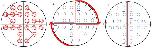
The circular scanning pattern involved walking each tree stem’s circumference to create complete cross-sections of the stem (Figure 1(a)). The figure-8 scanning pattern involved walking along the inside axes and half of the outside circumference of the plot, to ensure as much of each tree stem was captured as possible while prioritizing the speed of acquisition (Figure 1(b)). The transect scanning method involved walking both axes of the plot twice, scanning perpendicularly to the plot in opposite directions each time (Figure 1(c)). The circular pattern prioritized detailed data, the transect method favored acquisition speed, and the figure-8 pattern sought to balance both.

The Cloth Simulation Filtering (CSF) plugin for CloudCompare, developed by Zhang et al. (2016), can be used to identify ground features in point clouds and interpolate the ground surface for areas without data. This algorithm is commonly used to segment ground features within LiDAR datasets (Lee et al. 2020; Liu et al. 2021; Yang et al. 2020; Yu et al. 2022).

There are many different curve-fitting algorithms capable of estimating DBH, four of which were examined in this scoping study. For ‘Pratt’s direct-least-squares circle fit’ and ‘Taubin’s direct-least-squares circle fit’, the points are assumed to represent a perfect circle (Chernov 2022a; Chernov 2022b; Pratt 1987; Taubin 1991). Circle-fitting algorithms have been found to produce very accurate estimates of DBH from iPad Pro LiDAR data in previous studies, such as Wang et al. (2021), Tatsumi et al. (2021), and Gülci et al. (2023). In ‘Taubin’s direct-least-squares ellipse fit’ and ‘Szpak’s ellipse fit with Sampson distance and modified Levenberg-Marquardt step’, the points are assumed to represent an ellipsoid (Chernov 2022c; Szpak 2016; Taubin 1991; Szpak et al. 2015). While diameter tapes and calipers used to estimate DBH manually assume tree stems to represent perfect circles, the irregular nature of tree stems curve leads to an over-estimation of actual diameter using circles to model the tree stem (Hunčaga et al. 2020; Moran and Williams 2002). Ellipse fitting algorithms were used by Gollob et al. (2021) to produce estimates of DBH with accuracies comparable or superior to those estimated with circle-fitting formulas. The formulas developed by Pratt (1987) and Taubin (1991) are algebraic fitting formulas, which plot circles or ellipses of radius R around the center point of the dataset (a, b) while minimizing the distance from each point in the dataset to the plotted curve; through a least-squares method (Chernov and Lesort 2005). The center points for each fitted curve were calculated as the average X and Y values for the dataset (Pratt 1987, Taubin 1991). To solve the least-squares method, it is necessary to minimize the following non-linear Gradient-weighted Algebraic Fit (GRAF; Equation 1(1) $$F_4\left(a,b,R\right)=\sum _{i=1}^n\frac{\left[\right(x_i-a{)}^2+(y_i-b{)}^2-R^2{]}^2}{(x_i-a{)}^2+(y_i-b{)}^2}$$(1) ) (Chernov and Lesort 2004; Turner 1974). (1) $$F_4\left(a,b,R\right)=\sum _{i=1}^n\frac{\left[\right(x_i-a{)}^2+(y_i-b{)}^2-R^2{]}^2}{(x_i-a{)}^2+(y_i-b{)}^2}$$(1)

Where a, b, represent the coordinates of the center of the fitted curve, x and y represent the X and Y coordinates of point i in the stem shapefile, and R is the radius.

The GRAF is approximated differently in Taubin’s and Pratt’s approaches (Chernov and Lesort 2005). In Pratt (1987), the GRAF is simplified by assuming that $(x_i-a{)}^2+(y_i-b{)}^2\approx R^2$ as follows (Equation 2(2) $$F_4^i\left(a,b,R\right)=R^{-2}\sum _{i=1}^n[(x_i-a{)}^2+(y_i-b{)}^2-R^2{]}^2\mathrm{ }$$(2) ): (2) $$F_4^i\left(a,b,R\right)=R^{-2}\sum _{i=1}^n[(x_i-a{)}^2+(y_i-b{)}^2-R^2{]}^2\mathrm{ }$$(2)

In Taubin (1991), the GRAF is approximated by averaging the GRAF denominator over 1 $\preccurlyeq i\preccurlyeq n$ (Chernov and Lesort 2004) (Equation 3(3) $$F_4^{\mathit{\text{ii}}}\left(a,b,R\right)=\left(\frac{1}{\sum (x_i-a{)}^2+(y_i-b{)}^2}\right)\text{x}\sum _{i=1}^n\left[\right(x_i-a{)}^2+(y_i-b{)}^2-R^2{]}^2\mathrm{ }$$(3) ). (3) $$F_4^{\mathit{\text{ii}}}\left(a,b,R\right)=\left(\frac{1}{\sum (x_i-a{)}^2+(y_i-b{)}^2}\right)\text{x}\sum _{i=1}^n\left[\right(x_i-a{)}^2+(y_i-b{)}^2-R^2{]}^2\mathrm{ }$$(3)

Pratt’s approximation better handles datasets where the full circumference is not present, while Taubin’s formula is seen as faster and more accurate if the full circumference is present (Chernov and Lesort 2005). Formulas 1 and 2 both fit curves to a data set of point coordinates using the least-squared method, which has previously been used to estimate DBH (Chiappini et al. 2022; Gollob et al. 2021; Gülci et al. 2023; Tatsumi et al. 2021; Wang et al. 2021).

Szpak’s ellipse fit is an iterative geometric fit that uses an implicit barrier to separate feasible elliptic regions and infeasible hyperbolic regions, and uses a direct algebraic ellipse fit as the starting point (Szpak et al. 2015). The adapted Levenberg-Marquardt algorithm used by Szpak’s ellipse fit searches for a solution by using the implicit barrier to guide subsequent attempts at plotting an ellipse toward the optimal solution (Szpak et al. 2015). This formula assumes any noise within the dataset (i.e., points not directly on the path of the optimal solution) follow a normal, Gaussian distribution about the optimal ellipse (Szpak et al. 2015). A disadvantage of this algorithm is that the fitting results may be depreciated ellipses or degenerated parabolas if the dataset has a large proportion of noise or is limited to a small area of the curve (Szpak et al. 2015).

However, a comprehensive study which simultaneously examines the impacts of different combinations of scanning patterns, processing methods, and curve-fitting formulas to estimate DBH is still needed.

Hence, this study is intended as a scoping study to compare different point cloud acquisition and processing methods developed based on existing literature to evaluate combinations of these options on the same sites directly and create an optimized workflow for the future study intended to carry out in a natural forests environment.

This study expands upon Wang et al. 2022, who applied a singular, static scan and manual data processing to data acquired with an iPad Pro 12^th Generation to estimate DBH in the 25^th Sideroad research plantation forest near Thunder Bay, ON, Canada. The specific objectives were: (1) compare different scanning patterns with the iPad Pro for acquiring point cloud data for estimating DBH; (2) explore various data processing methods to extract DBH from the point cloud; and (3) identify the combination of acquisition and processing methods providing the most accurate estimates of DBH; and, (4) recommend a procedure for using iPad Pro LiDAR to estimate DBH.

Study area

Study area

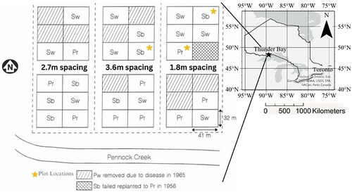
The study was conducted in a research plantation forest, known as the 25^th Sideroad Spacing Trial, near Thunder Bay, Ontario (48.37°N, 89.39°W) (Appendix 1). The Ontario Ministry of Natural Resources and Forestry (OMNRF) established the plantation in 1950 and has continuously managed the site (McClain et al. 1994). No stand tending operations have taken place. The trial comprises several blocks of different tree species, planted at different initial spacing distances. Three circular plots with a diameter of 10 m were selected for this study, with the following characteristics: (a) Plot ‘Pr’, Red Pine (Pinus resinosa) with 1.8 m spacing, planted with a density of 3082 stems/ha; (b) Plot ‘Sb’, Black Spruce (Picea mariana) with 3.6 m spacing, planted with a density of 771 stems/ha; and (c) Plot ‘Sb2’, Black Spruce (Picea mariana) with 1.8 m spacing, planted with a density of 3082 stems/ha.For our study, we only used data acquired for the plots marked with a gold star in Appendix 1. Below, Figure 2 shows the site conditions for plots Pr (Figure 2(a)), Sb (Figure 2(b)), and Sb2 (Figure 2(c)).

Figure 2. Images of the stands where plots Pr (a), Sb (b), and Sb2 (c) were performed.

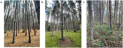
There was no understory or ingrowth in the Pr and Sb sites, while there was some understory and ingrowth in the Sb2 site (Figure 2(c)).

Methods

Data acquisition

Plot centers were randomly located within each selected stand, and marked using a meter stick with orange flagging tape. These plots were 10 m in diameter, corresponding to an area of 78.54 m². Each tree in a plot was assigned a number, ‘Tree 1′ being the tree closest to the plot center bearing northeast. Tree position within each plot was recorded manually with a compass and measuring tape as the distance (m) and bearing (degrees) from the plot center to the nearest point on each tree stem. The DBH of each tree in each plot was then measured manually (with a diameter tape) for validation. LiDAR data was acquired for each plot using the iOS application Zappcha with an iPad Pro 12^th Generation LiDAR scanner, using three different walking patterns (Circular, Figure-8, Transect) while scanning (Apple Inc. 2020; Veesus 2022). The LiDAR device was in continuous motion for the tested scanning patterns while capturing data.

As the circular scanning pattern captured many points, leading to large file sizes, it was necessary to divide each plot into four quadrants (Northeast, Southeast, Southwest, Northwest) and capture individual point clouds for each quadrant. Among the point cloud capture methods available in the Zappcha app, the ‘continuous scanning’ option was used for this project as this option allowed the greatest maximum scanning range (5 m; Veesus 2022). The other methods available (burst scan, timed scan) did not capture data continuously, and did so at a maximum scanning range of 2 m.

Since the visited stands were established in 1950, tree mortality has resulted in stand densities differing from the initial stand densities. As a result, the observed stand density (stems/ha) was calculated using the number of trees in each plot.

Point cloud processing

Raw point clouds acquired at the site were saved to the Zappcha Cloud service and later imported to the CloudCompare software for further processing (Girardeau-Montaut 2022; Veesus 2022).

The point clouds were projected using ArcGIS Pro, and areas of the point cloud that fell outside plot boundaries were removed (ESRI 2022). The Point clouds acquired with the circular scanning pattern for each quadrant of a plot were combined. Outliers were removed from each point cloud in CloudCompare software with the 'Statistical Outlier Removal (SOR)' tool (Girardeau-Montaut 2022). The SOR tool calculates the mean distance from each point in a point cloud to the nearest k neighbors and preserves points within a range of n standard deviations plus the mean neighbor distance for the dataset (k = 6 and n = 1; Girardeau-Montaut 2022). CSF was used to identify the ground elevation of each site, and extract cross-sections of the point cloud centered 1.3 m above the identified ground elevation with thicknesses of both 4 cm and 10 cm. These sizes were selected to account for an error of up to 1 cm in estimating the breast height elevation due to the cloth mesh resolution and classification threshold, as well as to evaluate the accuracy of different cross-section sizes.

For the single slice method, point cloud cross-sections were centered 1.3 m above ground. Based on the methods used by Liu et al. (2021), DBH was also estimated using the average diameter of each stem at multiple heights. The cross-sections used for this method were centered at 0.7 m, 1.0 m, 1.3 m, 1.6 m, and 1.9 m above the ground. The cross-sections at 0.7 m and 1.9 m were considered a pair, as were those at 1.0 m and 1.6 m. For both single- and multiple-cross-section methods, cross-sections of 4 cm and 10 cm thickness were extracted, and rasterized with a spatial resolution of 0.05 cm. These rasters showed a circular/elliptic pattern representing individual trees. For further processing, these raster files were converted to point shapefiles.

Extracting cross-sections

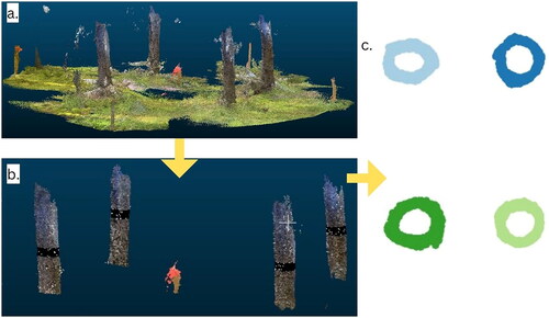
Points representing individual trees in the shapefiles were identified and segmented using density-based clustering (DBSCAN) in ArcGIS Pro, which can detect clusters of points with arbitrary geometries in two or more dimensions (ESRI 2023; Wang et al. 2019). Each unique cluster identified by this tool was segmented into a separate shapefile (ESRI 2023). Figure 3 shows a summary of this process for plot ‘Sb’, showing a point cloud acquired with the circular scanning method and clipped to plot boundaries (Figure 3a), the non-ground features point cloud with points in a single 4 cm cross-section at breast height highlighted in black (Figure 3b), as well as the DBSCAN output identifying unique clusters of points in each cross-section, with each cluster shown in a unique color and representing a single tree (Figure 3c).

Figure 3. Processing summary for Plot ‘Sb’: (a) point cloud acquired with circular scanning pattern; (b) filtered non-ground point cloud with single 4cm cross-section at breast height highlighted in black; and (c) clusters of points representing individual trees identified by HBDSCAN, with each colour representing a different tree.

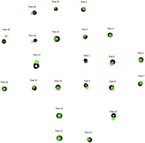
In order to pair the shapefiles created for each tree cross-section with the validation dataset for that tree, stem maps were created showing the position of each tree stem within each plot. These stem maps scaled tree stems according to the measured DBH for, as well as numbering each tree to facilitate pairing with the shapefile representing that tree. Figure 4 shows the stem map created for Plot ‘Pr’ in green, as well as a single 4 cm cross-section acquired with the circular scanning pattern for each tree.

Figure 4. Stem map for Plot ‘Pr’ (Green) and the DBSCAN output showing how the validation data was paired to the corresponding tree shapefile.

Estimating DBH

X and Y coordinates for each point in the shapefiles were appended to the file attribute tables for the shapefiles representing individual trees. For the multiple slice methods, if no points for a tree were present at a given height, the shapefile representing cross-section at the paired height was removed to minimize the estimate bias. The attribute table for each tree shapefile was exported to MathWorks (2022).

Four algebraic curve-fitting formulas were applied to the X and Y coordinates of the points in each tree shapefile to estimate the diameter of the cross-section. The diameters estimated with each of the four fitting functions were averaged for each tree. For the multiple slice methods, DBH was calculated as the average of the diameter estimates for all cross-sections of a given tree. If no points were present for a given tree at a certain height, the DBH estimate from the paired height were discarded to prevent skewing estimates.

Accuracy assessment

The estimated DBH values for each tree were compared with the field-measured DBH using two metrics. Absolute error (Difference between field-measured DBH and estimated DBH in cm) was calculated for each tree. Root Mean Square Error (RMSE) and relative Root Mean Square Error (rRMSE; RMSE as a percentage of the mean DBH value of the individual plot) were calculated for each unique combination of plot, scanning pattern, cross-section count, cross-section size, and curve-fitting formula.

Exploratory data analysis was done for individual tree absolute error values (LiDAR estimated DBH and field measurements) to check whether they were normally distributed. As they were not normally distributed, Kruskal-Wallis tests were performed to test if scanning pattern, cross-section count, cross-section size, or curve-fitting formula had statistically significant impacts on individual tree absolute error. Tests were also performed for each combination of two or more of the above independent variables. This also quantified the significance of each independent variable or pairwise interaction between two or more independent variables. Additionally, a Kruskal-Wallis test was performed to determine the significance of the relationship between stand density (stems/ha) and estimate accuracy (Individual tree absolute error).

Results

Validation data

Table 2 presents the number of trees measured in each plot, as well as the initial and observed site densities and the mean measured DBH for each plot.

Table 2. Characteristics of each field plot.

Plot	Number of Trees	Initial Stand Density (stems/ha)	Observed Stand Density (stems/ha)	Mean Measured DBH (cm)
Pr	22	3082	2801	21.71
Sb	4	3082	2037	25.53
Sb2	16	771	509	14.69

DBH estimation

Table 3 displays the minimum, mean, and maximum estimated DBH values (averaged for each combination of scan pattern, cross-section size, cross-section count, and curve-fitting formula) for each plot, as well as the mean measured DBH. This highlights the range of deviation about the mean measured DBH for each plot.

Table 3. Mean measured DBH and minimum, mean, and maximum estimated DBH (cm) for each plot with associated estimation methods.

Plot	Number of Trees	Mean measured DBH (cm)	Estimated DBH (cm)
			Minimum	Mean	Maximum
Pr	22	21.71	15.93 Transect scan, multiple 4cm CS, Taubin’s direct ellipse fit	20.88	23.01 Transect scan, single 4cm CS, Pratt’s direct circle fit
Sb	4	25.53	22.55 Figure-8 scan, single 10cm CS, Szpak’s ellipse fit	25.28	28.01 Transect scan, multiple 4cm CS, Pratt’s direct circle fit
Sb2	16	14.69	9.04 Figure-8 scan, single 4cm CS, Taubin’s direct ellipse fit	14.08	16.86 Circle scan, multiple 10cm CS, Pratt’s direct circle fit

Table 4 presents the distribution of the individual tree absolute error values by scanning pattern, showing the minimum, 1^st quartile, median, mean, 3^rd quartile, and max absolute errors (cm) achieved by any processing method.

Table 4. Distribution of absolute error (cm) values by scanning pattern.

Scanning Pattern	Min.	1^st Qu.	Median	Mean	3^rd Qu.	Max
Circular	0.00	0.53	1.05	1.51	1.80	10.26
Figure-8	0.16	0.90	1.86	2.84	3.63	24.32
Transect	0.00	0.79	2.01	3.16	4.33	27.52

Evaluating the significance of different experimental factors

Table 5 presents the results of Kruskal-Wallis tests that were used to determine the level of statistical significance that the tested scanning patterns, cross-section counts, cross-section sizes, and curve-fitting formulas had on DBH estimate accuracy (individual tree absolute error). Results were reported individually for each independent variable and for interactions between two or more independent variables with a moderate or significant magnitude of effect.

Table 5. Kruskal-Wallis test results testing the significance of scanning pattern, cross-section size, cross-section count, and curve-fitting formula on individual tree absolute error.

Factor(s)	Df	Test Statistic	p-value	Effect Size	Magnitude
Scanning pattern	2	149.12	4.16^-33	0.075	Moderate
Cross-Section Size	1	3.97	0.05	0.002	Small
Cross-Section Count	1	12.89	3.31^-04	0.006	Small
Fitting Formula	4	29.78	5.43^-06	0.013	Small
Scan pattern x CS Size	5	162.04	3.64^-33	0.080	Moderate
Scan pattern x CS Count	5	188.48	8.26^-39	0.094	Moderate
Scan Pattern x Fitting Formula	14	213.83	8.13^-38	0.103	Moderate
Scan pattern x CS Size x CS Count	11	204.28	9.64^-38	0.099	Moderate
Scan pattern x CS Size x Fitting Formula	29	229.01	5.69^-33	0.104	Moderate
Scan pattern x CS Size x CS Count x Fitting Formula	59	282.97	5.40^-31	0.118	Moderate

*CS = Cross-Section.

The results highlight that the scanning pattern had a moderate effect on individual tree absolute error. Cross-section size, cross-section count, and fitting formula had small effects on the accuracy of the DBH estimates. All two- or three-way interactions involving scan patterns also had moderate magnitudes of effect. As the scanning pattern was the only independent variable to have a moderate effect on absolute error on its own, a Dunn-Bonferroni test was conducted to determine the significances of differences between scanning methods.

As Table 6 shows, the circular scanning pattern resulted in estimate accuracies significantly different from those of both the figure-8 and transect scanning patterns, while the figure-8 and transect scanning patterns did not significantly differ in their effects on estimate accuracy.

Table 6. Dunn-Bonferroni test results showing statistical significances of differences between scanning methods.

Group 1	Group 2	Statistic	Adjusted p-Value	Adjusted Significance
Circle	Figure-8	8.53	4.29^-17	< 0.001
Circle	Transect	11.30	1.09^-29	< 0.001
Figure-8	Transect	0.51	0.61	Not Significant

In addition to the tested independent variables, a Kruskal-Wallis test was also performed to test the significance of observed stand density on estimated DBH accuracy.

Table 7 shows that the observed stand density had a small impact on the accuracy of DBH estimates. Table 8 compares the individual tree absolute error values (cm and %), averaged across all plots and curve-fitting formulas for each combination of scanning pattern, cross-section count, and cross-section size. The circle scanning pattern provided the most accurate DBH estimates, and the transect pattern provided the least accurate DBH estimates. When using the circle scanning pattern, the single 4 cm cross-section led to the most accurate estimates, while the multiple 10 cm cross-sections led to the most accurate estimates in both figure-8 and transect patterns.

Table 7. Kruskal-Wallis results showing the significance of stand density on individual tree absolute error.

Factor	Df	Test Statistic	p-value	Effect Size	Magnitude
Stand Density	2	26.36	1.89^-06	0.012	Small

Table 8. Mean absolute error at the individual tree level as a function of the scanning pattern, cross-section count, and cross-section size. Bold figures represent the optimal combination for each scanning pattern.

Scanning pattern	Cross-Section Count	Cross-Section Size (cm)	Mean Absolute Error (cm)	Relative Error (%)
Circle	Single	4	0.99	5.11
	Single	10	1.35	6.95
	Multiple	4	1.90	9.80
	Multiple	10	1.79	9.22
Figure-8	Single	4	3.51	21.00
	Single	10	2.77	16.53
	Multiple	4	2.72	16.24
	Multiple	10	2.38	13.92
Transect	Single	4	3.57	21.34
	Single	10	2.60	21.34
	Multiple	4	3.32	17.08
	Multiple	10	3.16	16.25

Table 9 presents the mean absolute error (cm and %) for each combination of scanning pattern and curve-fitting formula, averaged across all plots, cross-section counts, and cross-section sizes.

Table 9. rRMSE (%) for each combination of scanning pattern and curve-fitting formula. Bold values indicate optimal rRMSE (%) for each scanning pattern.

Scanning pattern	Curve-Fitting Formula	Mean Absolute Error (cm)	Relative Error (%)
Circular	Pratt’s Direct-Least Squares Circle	1.56	8.03
	Taubin’s Direct-Least Squares Circle	1.33	6.85
	Taubin’s Direct-Least Squares Ellipse	1.48	7.62
	Szpak’s Ellipse Fit with Sampson Method	1.81	9.35
	Combined Formula	1.36	6.99
Figure-8	Pratt’s Direct-Least Squares Circle	2.15	12.81
	Taubin’s Direct-Least Squares Circle	2.37	14.07
	Taubin’s Direct-Least Squares Ellipse	3.43	20.40
	Szpak’s Ellipse Fit with Sampson Method	3.82	22.74
	Combined Formula	2.40	14.30
Transect	Pratt’s Direct-Least Squares Circle	2.60	15.48
	Taubin’s Direct-Least Squares Circle	2.58	15.48
	Taubin’s Direct-Least Squares Ellipse	4.32	22.10
	Szpak’s Ellipse Fit with Sampson Method	3.76	19.27
	Combined Formula	2.54	12.98

As stands in a natural forest will vary in density (stems/ha), a weighted average of RMSE was calculated for the three plots as follows: $$\text{Average RMSE}=\left[\left(\text{22 trees}*\text{Plot}‘\text{Pr}’\text{mean RMSE}\right)+\left(\text{4 trees}*\text{Plot}‘\text{Sb}’\text{mean RMSE}\right)+\left(\text{16 trees}*\text{Plot}‘\text{Sb}2’\text{mean RMSE}\right)\right]/\text{42 trees}.$$

Table 10 presents the average and optimal RMSE (in cm) and the rRMSE for each scanning pattern, averaged for all plots, cross-section counts, cross-section sizes, and curve-fitting formulas. It shows the circular scanning pattern, using a single 4 cm cross-section and a combination of all four curve-fitting formulas as the combination of data acquisition and processing methods provides the most accurate estimates of DBH. The use of a single 4 cm cross-section with Pratt’s direct least-squares circle fit led to the most accurate estimates of DBH with the figure-8 scanning pattern. Processing the data with multiple 4 cm cross-sections and a combination of all tested curve-fitting formulas provided the most accurate estimates of DBH for the transect scanning pattern.

Table 10. Average and optimal RMSE (cm) and rRMSE as a function of the scanning pattern.

Scanning pattern	RMSE (cm)		rRMSE (%)		Estimation method producing the optimal RMSE
	Mean	Optimal	Mean	Optimal
Circular	2.01	1.13	11.24	6.17	Average of all formulas & single 4cm CS.
Figure-8	3.85	1.68	24.52	10.17	Pratt’s least-squares circle fit & single 4cm CS.
Transect	4.29	3.12	23.86	17.05	Average of all formulas & multiple 4cm CS.

In order to model the relationship between actual and estimated DBH, these values for all trees were plotted with a line showing a 1:1 relationship (Figure 5). Figure 5 shows that the circular scanning pattern produced estimates consistently near the line modeling the 1:1 relationsghips, with outliers coming from the figure-8 or transect scanning patterns using single cross-sections.

Figure 5. Estimated DBH (cm) as a function of Actual DBH (cm) by Scanning Method and number of Cross-Sections with plotted line showing a 1:1 relationship.

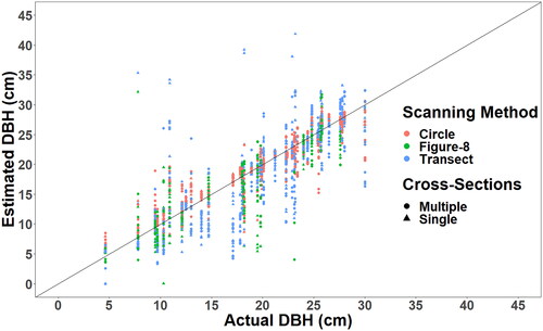
Based on Figure 5, the circular scanning pattern produced most accurate estimates of DBH across the range of actual DBH values present in the data. Figure-8 and transect scanning patterns resulted in the majority of the outliers, especially when only one stem cross-section was used.

Scanning errors with iPad Pro LiDAR

Due to the nature of the walking path for the transect scanning pattern (Figure 2c), each tree was scanned on two separate passes around the plot, potentially causing accumulated positioning errors. The literature shows there are known Inertial Measurement Unit (IMU) drift, rotational, and GPS positional errors with the iPad Pro LiDAR scanner that may cause issues in acquired point clouds (Corradetti et al. 2022; Tavani et al. 2022; Wang et al. 2021). An example of this is highlighted in Figure 6, which shows the top view of the 4 cm single cross-sections of the same tree in the Sb plot for different scanning patterns: circular (6a), figure-8(6b), and transect (6c).

Figure 6. Top-down images of single 4cm tree cross-sections acquired with the (a) circular; (b) figure-8; and (c) transect scanning patterns.

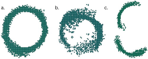
As seen in Figure 6a, the circular scanning pattern resulted in a cross-section showing the entire circumference of the tree with few outliers. The figure-8 scanning pattern (Figure 6b) resulted in a cross-section representing most of the stem circumference, with some outliers. The transect scanning pattern (Figure 6c) showed a cross-section consisting of two separate sections, each of which represented only half of the stem’s circumference, indicating some locational errors.

Figure 7 shows cross-sections of Tree 9 in Plot ‘Pr’, extracted from point clouds acquired with the circular scanning pattern (a) and transect scanning pattern (b). For both cross-sections, the tree centroid point and results of Pratt’s circle fit (Red line) and Szpak’s ellipse fit (Blue line) are shown.

Figure 7. Plotted stem cross-sections and centroid points (black circle) extracted from a circular scanning pattern point cloud (a) and a transect scanning pattern point cloud (b), with plotted results for Pratt’s circle fit (red) and Szpak’s ellipse fit (blue).

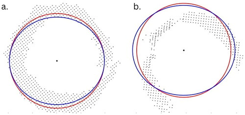
As Figure 7 shows, the circular scanning pattern provided a feasible stem centroid location, while the transect pattern did not. Additionally, the fitted curves aligned with the stem cross-section extracted from the circular scanning pattern but not the transect cross-section.

Discussion

DBH estimation accuracy

The circular scanning pattern produced the lowest optimal and average absolute error (Table 10), while also resulting in the lowest overall values for individual tree absolute error (Table 4). Due to the irregular and inconsistent shapes of tree stems, the greater the distribution of stem points about the circumference of each tree in the point cloud, the more accurate the estimates of DBH were (Hunčaga et al. 2020). When a combination of circle- and ellipse-fitting formulas were applied to a single 4 cm cross-section, an RMSE of 1.13 cm (rRMSE of 6.17%) was achieved. This method produced a lower RMSE value than those reported in many other studies using the iPad Pro LiDAR scanner for DBH estimation. For example, Gollob et al. (2021) report RMSE (rRMSE) values between 3.13 cm (10.50%; ellipse fit) and 6.29 cm (21.23%; cylinder fit) using the Polycam and SiteScape iOS Applications for an iPad Pro 12^th Generation. They applied ellipse- and cylinder-fitting formulas to 15 cm cross-sections and were able to acquire point clouds with a scanning pattern similar to the circular scanning pattern (Figure 2a) used in this study. Wang et al. (2021) reported RMSE (rRMSE) values between 2.78 cm (7.27%) and 5.18 cm (13.03%) in an urban forest using the 3D Scanner iOS application for the iPad Pro to acquire data, using the optimal circle fit formula in DendroCloud to extract DBH. Chiappini et al. (2022) achieved RMSE (rRMSE) values of 4.1 cm (16.3%) with the 3D Forest iOS application, 6.8 cm (27.0%) with the VoxR package in R, and 2.7 cm (10.0%) using a convex hull fit with the “TreeLS-lidr-rLiDAR” package in R. Tatsumi et al. (2021) achieved RMSE (rRMSE) values of 2.3 cm (10.3%) using the ForestScanner iOS Application on an iPhone 13 Pro and 2.3 cm (10.5%) using the same application with an iPad Pro 2021. A previous study at the 25^th Sideroad Site obtained RMSE (rRMSE) values between 2.82 cm (12.82%) and 5.9 cm (26.82%) by manually fitting curves to point clouds acquired with the iPad Pro 12^th Generation (Wang et al. 2022).

Our method did generate results comparable to those achieved with higher-quality terrestrial LiDAR scanners. For example, Liu et al. (2021) report RMSE (rRMSE) values between 1.97 cm (6.35%; urban forest) and 3.17 cm (13.21%; natural forest) using a Velodyne VLP-16 LiDAR sensor, with a range of up 100 m and an accuracy of ±3 cm. In their study, they used a RANSAC circle-fitting formula applied to 7 stem cross-sections. In another study, Gollob et al. (2021) report RMSE (rRMSE) values of 1.59 cm (6.29%; circle fit) to 2.07 cm (8.29%; cylinder fit) using a GeoSLAM ZEB HORIZON scanner with a maximum range of 100 m and an accuracy of ±3 cm. Our results support previous findings that the circular scanning pattern results in the most accurate DBH estimates (i.e., with the lowest rRMSE values). The circular scanning pattern also resulted in more consistent DBH estimation accuracies, with a lower maximum error than the other scanning patterns (Table 4).

For the circular scanning pattern, both tested single cross-section methods were more accurate than the multiple cross-section methods for all tested plots. For the figure-8 and transect scanning patterns, the multiple cross-section methods did, however, lead to improved DBH estimate accuracy. This is consistent with the findings of Liu et al. (2021), who observed improved DBH estimate accuracy using multiple stem-cross sections in comparison to single cross-sections.

Our study allows to conclude that the circular scanning pattern, using a combination of different curve-fitting formulas applied to a single 4 cm cross-section of the stem represents the optimal combination for extracting DBH using iPad Pro LiDAR sensor.

Scanning errors with iPad Pro LiDAR

The irregular geometry of tree stems, the presence of noise (i.e., points in a point cloud that did not represent features in the correct location), IMU drift, and rotational erros within the acquired point clouds are possible explanations for the low accuracy for the figure-8 and transect scanning patterns. Szpak et al. (2015) noted that at least 400 points representing 50% or more of the curve circumference were necessary for their ellipse fit to produce reliably accurate results. Many cross-sections extracted from point clouds acquired with the transect scanning pattern tend to have fewer than 200 points, with less than 50% of the stem circumference being represented. The figure-8 scanning pattern offered an improvement over the transect pattern with respect to both the number of points associated with each tree stem cross-section and in the proportion of tree circumference represented. However, both patterns resulted in a greater number of inaccurate placement of points in the acquired datasets (Figure 7b and c) compared to those of the circular scanning pattern (Figure 7a).

Positional errors, caused by factors such as Inertial Measurement Units (IMUs) or the device GPS, may have contributed to inaccurate location of acquired points with the iPad Pro LiDAR scanner (Luetzenburg et al. 2021). Previous studies have found iPad and iPhone LiDAR scans result in “crude” 3-dimensional models with low surface fidelity due to accumulated IMU errors (Tavani et al. 2022; Corradetti et al. 2022). Over the course of a scan, previous studies have found the factor by which points are incorrectly located within a cloud to reach up to 2 m (Castel and D’Hoedt 2022). While Tavani et al. (2019) suggest the use of multiple ground control points and post-processing to correctly align and scale point clouds, this was not performed in this study, potentially contributing to the observed errors.

The four curve-fitting formulas used in this determined the centroid coordinates (a, b) of each fitted curve as the average X and Y values in each dataset (Pratt 1987; Taubin 1991; Szpak et al. 2015). As a result, increasing the proportion of noise points within each tree cross-section was found to correspond with an increase in the misplacement of the stem centroid.

Impact of stand density

In this study, a Kruskal-Wallis test showed that site density had a small impact (p-value =1.89 × 10⁻⁶, effect size = 0.012) on estimate accuracy. This was a greater significance than the cross-section sizes and counts, but less significant than the scanning pattern or fitting formula used. There was additionally no observed pattern in the interaction between stand density and estimate accuracy. In a study regarding initial tree spacing and DBH at the study site, McClain et al. (1994) observed a highly significant difference (p < 0.01) in DBH values between initial spacing distances. Based on this result, a regression was performed, testing the relationship between individual tree size and estimate accuracy. A strong, positive correlation was observed between estimate accuracy and increases in measured DBH (cm, R = 0.98), which is consistent with previous findings (Chen et al. 2022; Liu et al. 2021; Wang et al. 2022). The differences between correlation versus causation in the relationships between stand density, measured stem size, and estimate accuracy were not explored.

Conclusions

This scoping study suggests that the circular scanning pattern with a single 4 cm cross-section and a combination of circle- and ellipse- fitting formulas produced the most accurate DBH values over a range of observed stand densities. RMSE values as low as 1.13 cm (6.17% of mean plot DBH) were achieved with this method. DBH estimate accuracy was found to have no correlation with site density (stems/ha; R²=0.18) and a strong positive correlation with increases in stem size (cm; R²=0.96).

Boreal forest landscapes continue to be dominated by natural (wildfire origin) stands, as opposed to uniformly-spaced, intensively managed plantations. Therefore, our future research to expand on the findings of this scoping study will extend to stands representing a range of natural boreal forest conditions to evaluate the feasibility, in terms of accuracy and efficiency, of DBH estimation. This research will include an examination of how different stand conditions such as the presence of understory vegetation (i.e., medium to tall shrubs), stand age (i.e., differences in horizontal and vertical complexities), and stand species composition (e.g., broadleaf- or conifer-dominant and mixed wood) impact the accuracy of DBH estimates. Further, a workflow for operationalizing the use of iPad Pro LiDAR for DBH estimation in forest inventories should also be developed.

Acknowledgments

The authors appreciate the Ontario Ministry of Natural Resources and Forestry for allowing data collection at the 25^th Sideroad Spacing Trial.

Disclosure statement

The authors reported no conflict of interest.

Data availability statement

Data are available through a request to the corresponding author.

Additional information

Funding

This research was partly funded by the "Research Development Fund" and "Start-up" funds of Dr. Muditha K. Heenkenda at Lakehead University, Ontario, Canada. Additional funding was received from a Graduate Assistantship with the Faculty of Natural Resources Management at Lakehead University, Ontario, Canada.

Appendix 1.

25th sideroad site map and plot locations

References

- Aijazi, A.K., Checchin, P., Malaterre, L., and Trassoudaine, L. 2017. “Automatic Detection and Parameter Estimation of Trees for Forest Inventory Applications Using 3D Terrestrial LiDAR.” Remote Sensing, Vol. 9 ((No. 9): pp. 946. Article 9 doi:10.3390/rs9090946.
- Apple 2020. Apple unveils new iPad Pro with LiDAR Scanner and trackpad support in iPadOS. Apple Newsroom. https://www.apple.com/newsroom/2020/03/apple-unveils-new-ipad-pro-with-lidar-scanner-and-trackpad-support-in-ipados/
- Bauwens, S., Bartholomeus, H., Calders, K., and Lejeune, P. 2016. “Forest Inventory with Terrestrial LiDAR: A Comparison of Static and Hand-Held Mobile Laser Scanning.” Forests, Vol. 7 (No. 12): pp. 127. Article 6 doi:10.3390/f7060127.
- Bilyk, A., Pulkki, R., Shahi, C., and Larocque, G.R. 2021. “Development of the Ontario Forest Resources Inventory: A historical review.” Canadian Journal of Forest Research, Vol. 51 (No. 2): pp. 198–209. doi:10.1139/cjfr-2020-0234.
- Blanco, A.C., Tamondong, A.M., Perez, A.M.C., Ang, M.R.C.O., and Paringit, E.C. 2015. “The PHIL-LiDAR 2 Program: National Forest Resource Inventory of the Phillipines using LiDAR and other Remotely Sensed Data.” The International Archives of the Photogrammetry, Remote Sensing and Spatial Information Sciences, Vol. XL-7/W3 pp. 1123–1127. doi:10.5194/isprsarchives-XL-7-W3-1123-2015.
- Brede, B., Lau, A., Bartholomeus, H.M., and Kooistra, L. 2017. “Comparing RIEGL RiCOPTER UAV LiDAR Derived Canopy Height and DBH with Terrestrial LiDAR.” Sensors (Basel, Switzerland), Vol. 17 (No. 10): pp. 2371. Article 10 doi:10.3390/s17102371.
- Calders, K., Adams, J., Armston, J., Bartholomeus, H., Bauwens, S., Bentley, L.P., Chave, J., et al. 2020. “Terrestrial laser scanning in forest ecology: Expanding the horizon.” Remote Sensing of Environment, Vol. 251 pp. 112102. doi:10.1016/j.rse.2020.112102.
- Castel, C., and D’Hoedt, M. 2022. Automated forest inventory using the iPad Pro LiDAR scanner [Masters]. Ecole Polytechnique de Louvain, Universite Cathiolique de Louvain.
- Chen, Q., Gao, T., Zhu, J., Wu, F., Li, X., Lu, D., and Yu, F. 2022. “Individual Tree Segmentation and Tree Height Estimation Using Leaf-Off and Leaf-On UAV-LiDAR Data in Dense Deciduous Forests.” Remote Sensing, Vol. 14 (No. 12): pp. 2787. Article 12 doi:10.3390/rs14122787.
- Chernov, N. 2022a. Circle Fit (Pratt method) (1.0.0) [MATLAB; Windows]. MathWorks. https://www.mathworks.com/matlabcentral/fileexchange/22643-circle-fit-pratt-method
- Chernov, N. 2022b. Circle Fit (Taubin method) (1.0.0) [MATLAB; Windows]. MathWorks. https://www.mathworks.com/matlabcentral/fileexchange/22678-circle-fit-taubin-method
- Chernov, N. 2022c. Ellipse Fit (Taubin Method) (1.0.0) [MATLAB; Windows]. MathWorks. https://www.mathworks.com/matlabcentral/fileexchange/22683-ellipse-fit-taubin-method
- Chernov, N., and Lesort, C. 2004. “Statistical efficiency of curve fitting algorithms.” Computational Statistics & Data Analysis, Vol. 47 (No. 4): pp. 713–728. doi:10.1016/j.csda.2003.11.008.
- Chernov, N., and Lesort, C. 2005. “Least squares Fitting of Circles.” Journal of Mathematical Imaging and Vision, Vol. 23 (No. 3): pp. 239–252. doi:10.1007/s10851-005-0482-8.
- Chiappini, S., Pierdicca, R., Malandra, F., Tonelli, E., Malinverni, E.S., Urbinati, C., and Vitali, A. 2022. “Comparing Mobile Laser Scanner and manual measurements for dendrometric variables estimation in a black pine (Pinus nigra Arn.) plantation.” Computers and Electronics in Agriculture, Vol. 198: pp. 107069. doi:10.1016/j.compag.2022.107069.
- Corradetti, A., Seers, T., Mercuri, M., Calligaris, C., Busetti, A., and Zini, L. 2022. “Benchmarking Different SfM-MVS Photogrammetric and iOS LiDAR Acquisition Methods for the Digital Preservation of a Short-Lived Excavation: A Case Study from an Area of Sinkhole Related Subsidence.” Remote Sensing, Vol. 14 (No. 20): pp. 5187. Article 20 doi:10.3390/rs14205187.
- Côté, J.-F., Fournier, R.A., and Egli, R. 2011. “An architectural model of trees to estimate forest structural attributes using terrestrial LiDAR.” Environmental Modelling & Software, Vol. 26 (No. 6): pp. 761–777. doi:10.1016/j.envsoft.2010.12.008.
- Dassot, M., Constant, T., and Fournier, M. 2011. “The use of terrestrial LiDAR technology in forest science: Application fields, benefits and challenges.” Annals of Forest Science, Vol. 68 (No. 5): pp. 959–974. Article 5 doi:10.1007/s13595-011-0102-2.
- ESRI 2023. ArcGIS Pro (3.10) [C++; Windows]. Redlands, United States of America: ESRI. esri.com/en-us/arcgis/products/arcgis-pro/overview
- Girardeau-Montaut, D. 2022. CloudCompare—Open Source project (2.12.4 Kyiv) [C++; Windows]. CloudCompare. https://www.cloudcompare.org/
- Girardeau-Montaut, D., and Rascale, P. 2022. CloudComPy: Python Wrapper for CloudCompare (2.12.4) [C++, Python; Windows]. CloudCompare (GPL). https://github.com/CloudCompare/CloudComPy
- Gollob, C., Ritter, T., Kraßnitzer, R., Tockner, A., and Nothdurft, A. 2021. “Measurement of Forest Inventory Parameters with Apple iPad Pro and Integrated LiDAR Technology.” Remote Sensing, Vol. 13 (No. 16): pp. 3129. Article 16 doi:10.3390/rs13163129.
- Gülci, S., Yurtseven, H., Akay, A.O., and Akgul, M. 2023. “Measuring tree diameter using a LiDAR-equipped smartphone: a comparison of smartphone- and caliper-based DBH.” Environmental Monitoring and Assessment, Vol. 195 (No. 6): pp. 678. doi:10.1007/s10661-023-11366-8.
- Hopkinson, C., Chasmer, L., Young-Pow, C., and Treitz, P. 2004. “Assessing forest metrics with a ground-based scanning LiDAR.” Canadian Journal of Forest Research, Vol. 34 (No. 3): pp. 573–583. doi:10.1139/x03-225.
- Hunčaga, M., Chudá, J., Tomaštík, J., Slámová, M., Koreň, M., and Chudý, F. 2020. “The Comparison of Stem Curve Accuracy Determined from Point Clouds Acquired by Different Terrestrial Remote Sensing Methods.” Remote Sensing, Vol. 12 (No. 17): pp. 2739. Article 17 doi:10.3390/rs12172739.
- Hyyppä, E., Hyyppä, J., Hakala, T., Kukko, A., Wulder, M.A., White, J.C., Pyörälä, J., et al. 2020. “Under-canopy UAV laser scanning for accurate forest field measurements.” ISPRS Journal of Photogrammetry and Remote Sensing, Vol. 164: pp. 41–60. doi:10.1016/j.isprsjprs.2020.03.021.
- Hyyppä, E., Yu, X., Kaartinen, H., Hakala, T., Kukko, A., Vastaranta, M., and Hyyppä, J. 2020. “Comparison of Backpack, Handheld, Under-Canopy UAV, and Above-Canopy UAV Laser Scanning for Field Reference Data Collection in Boreal Forests.” Remote Sensing, Vol. 12 (No. 20): pp. 3327. Article 20 doi:10.3390/rs12203327.
- Lee, J.B., Jung, J.H., and Kim, H.J. 2020. “Segmentation of Seabed Points from Airborne Bathymetric LiDAR Point Clouds Using Cloth Simulation Filtering Algorithm.” Journal of the Korean Society of Surveying, Geodesy, Photogrammetry and Cartography, Vol. 38 (No. 1): pp. 1–9. doi:10.7848/ksgpc.2020.38.1.1.
- Liang, X., Hyyppä, J., Kaartinen, H., Lehtomäki, M., Pyörälä, J., Pfeifer, N., Holopainen, M., et al. 2018. “International benchmarking of terrestrial laser scanning approaches for forest inventories.” ISPRS Journal of Photogrammetry and Remote Sensing, Vol. 144 pp. 137–179. doi:10.1016/j.isprsjprs.2018.06.021.
- Liu, G., Wang, J., Dong, P., Chen, Y., and Liu, Z. 2018. “Estimating Individual Tree Height and Diameter at Breast Height (DBH) from Terrestrial Laser Scanning (TLS) Data at Plot Level.” Forests, Vol. 9 (No. 7): pp. 398. Article 7 doi:10.3390/f9070398.
- Liu, L., Zhang, A., Xiao, S., Hu, S., He, N., Pang, H., Zhang, X., and Yang, S. 2021. “Single Tree Segmentation and Diameter at Breast Height Estimation with Mobile LiDAR.” IEEE Access., Vol. 9: pp. 24314–24325. doi:10.1109/ACCESS.2021.3056877.
- Lovell, J.L., Jupp, D.L.B., Culvenor, D.S., and Coops, N.C. 2003. “Using airborne and ground-based ranging lidar to measure canopy structure in Australian forests.” Canadian Journal of Remote Sensing, Vol. 29 (No. 5): pp. 607–622. doi:10.5589/m03-026.
- Luetzenburg, G., Kroon, A., and Bjørk, A.A. 2021. “Evaluation of the Apple iPhone 12 Pro LiDAR for an Application in Geosciences.” Scientific Reports, Vol. 11 (No. 1):Article 22221. doi:10.1038/s41598-021-01763-9.
- MathWorks 2022. MATLAB (r2022b) [C/C++]. Natick, United States of America: The MathWorks, Inc. https://www.mathworks.com/products/matlab.html
- McClain, K.M., Morris, D.M., Hills, S.C., and Buse, L.J. 1994. “The effects on initial spacing on growth and crown development for planted northern conifers: 37-year results.” Forestry Chronicle., Vol. 70 (No. 2): pp. 174–182. doi:10.5558/tfc70174-2.
- Moran, L.A., and Williams, R.A. 2002. “Comparison of Three Dendrometers in Measuring Diameter at Breast Height.” Northern Journal of Applied Forestry, Vol. 19 (No. 1): pp. 28–33. doi:10.1093/njaf/19.1.28.
- Müller, A., Olschewski, R., Unterberger, C., and Knoke, T. 2020. “The valuation of forest ecosystem services as a tool for management planning – A choice experiment | Elsevier Enhanced Reader.” Journal of Environmental Management, Vol. 271 pp. 111008. doi:10.1016/j.jenvman.2020.111008.
- [OMNRF] Ontario Ministry of Natural Resources and Forestry 2015. Forest Management Guide to Silviculture in the Great Lakes-St. Lawrence and Boreal Forests of Ontario. Queen’s Printer for Ontario.
- [OMNRF] Ontario Ministry of Natural Resources and Forestry 2021. Vegetation Sampling Network Protocol: Technical specifications for field plots. Ontario Ministry of Natural Resources and Forestry, Science and Research Branch, Peterborough, ON. Science and Research Technical Manual TM-10. 173pp. + appendices.
- Pfeifer, N., and Winterhalder, D. 2004. “Modelling of Tree Cross Sections from Terrestrial Laser Scanning Data with Free-Form Curves.” International Archives of Photogrammetry, Remote Sensing, and Spatial Information Sciences, Vol. 36 (No. 8): pp. 76–81.
- Pratt, V. 1987. “Direct least-squares fitting of algebraic surfaces | Proceedings of the 14th annual conference on Computer graphics and interactive techniques.” ACM SIGGRAPH Computer Graphics, Vol. 21 (No. 4): pp. 145–152. ACM-0-89791-227-6/87/007/0145 doi:10.1145/37401.37420.
- Szpak, D. Z. L. 2016. Guaranteed Ellipse Fitting with a Confidence Region and an Uncertainty Measure for Centre, Axes and Orientation [Matlab]. https://github.com/zygmuntszpak/guaranteed-ellipse-fitting-with-a-confidence-region-and-an-uncertainty-measure (Original work published 2015)
- Szpak, Z.L., Chojnacki, W., and van den Hengel, A. 2015. “Guaranteed Ellipse Fitting with a Confidence Region and an Uncertainty Measure for Centre, Axes, and Orientation.” Journal of Mathematical Imaging and Vision, Vol. 52 (No. 2): pp. 173–199. doi:10.1007/s10851-014-0536-x.
- Tatsumi, S., Yamaguchi, K., and Furuya, N. 2021. “ForestScanner: A mobile application for measuring and mapping trees with LiDAR-equipped iPhone and iPad.” Methods in Ecology and Evolution, Vol. 14 (No. 7): pp. 1603–1609. doi:10.1111/2041-210X.13900.
- Taubin, G. 1991. “Estimation of planar curves, surfaces, and nonplanar space curves defined by implicit equations with applications to edge and range image segmentation.” IEEE Transactions on Pattern Analysis and Machine Intelligence, Vol. 13 (No. 11): pp. 1115–1138. doi:10.1109/34.103273.
- Tavani, S., Corradetti, A., Granado, P., Snidero, M., Seers, T.D., and Mazzoli, S. 2019. “Smartphone: An alternative to ground control points for orienting virtual outcrop models and assessing their quality.” Geosphere, Vol. 15 (No. 6): pp. 2043–2052. doi:10.1130/GES02167.1.
- Tavani, S., Billi, A., Corradetti, A., Mercuri, M., Bosman, A., Cuffaro, M., Seers, T., and Carminati, E. 2022. “Smartphone assisted fieldwork: Towards the digital transition of geoscience fieldwork using LiDAR-equipped iPhones.” Earth-Science Reviews, Vol. 227 pp. 103969. doi:10.1016/j.earscirev.2022.103969.
- Turner, K. 1974. Computer perception of curved objects using a television camera. Ph.D. Thesis, Dept. of Machine Intelligence, University of Edinburgh.
- Veesus 2022. ZAPPCHA: Mobile LiDAR Scanner (5.6) [Swift; IOS]. Hastings, United Kingdom: Veesus. https://zappcha.com/
- Wang, C., Ji, M., Wang, J., Wen, W., Li, T., and Sun, Y. 2019. “An Improved DBSCAN Method for LiDAR Data Segmentation with Automatic Eps Estimation.” Sensors (Basel, Switzerland), Vol. 19 (No. 1): pp. 172. doi:10.3390/s19010172.
- Wang, X., Singh, A., Pervysheva, Y., Lamatungga, K.E., Murtinová, V., Mukarram, M., Zhu, Q., Song, K., Surový, P., and Mokroš, M. 2021. “Evaluation of iPad Pro 2020 LiDAR for Estimating Tree Diameters in Urban Forest.” ISPRS Annals of the Photogrammetry, Remote Sensing and Spatial Information Sciences, Vol. VIII-4/W1-2021 pp. 105–110. doi:10.5194/isprs-annals-VIII-4-W1-2021-105-2021.
- Wang, F., Heenkenda, M.K., and Freeburn, J.T. 2022. “Estimating tree Diameter at Breast Height (DBH) using an iPad Pro LiDAR sensor.” Remote Sensing Letters, Vol. 13 (No. 6): pp. 568–578. doi:10.1080/2150704X.2022.2051635.
- White, J.C., Coops, N.C., Wulder, M.A., Vastaranta, M., Hilker, T., and Tompalski, P. 2016. “Remote Sensing Technologies for Enhancing Forest Inventories: A Review.” Canadian Journal of Remote Sensing, Vol. 42 (No. 5): pp. 619–641. doi:10.1080/07038992.2016.1207484.
- Wickham, H. 2016. ggplot2: Elegant Graphics for Data Analysis (1st ed.). Berlin, Germany: Springer-Verlag. ggplot2.tidyverse.org
- Woods, M., Pitt, D., Penner, M., Lim, K., Nesbitt, D., Etheridge, D., and Treitz, P. 2011. “Operational implementation of a LiDAR inventory in Boreal Ontario.” The Forestry Chronicle, Vol. 87 (No. 04): pp. 512–528. doi:10.5558/tfc2011-050.
- Yang, A., Wu, Z., Yang, F., Su, D., Ma, Y., Zhao, D., and Qi, C. 2020. “Filtering of airborne LiDAR bathymetry based on bidirectional cloth simulation.” ISPRS Journal of Photogrammetry and Remote Sensing, Vol. 163 pp. 49–61. doi:10.1016/j.isprsjprs.2020.03.004.
- Yu, D., He, L., Ye, F., Jiang, L., Zhang, C., Fang, Z., and Liang, Z. 2022. “Unsupervised ground filtering of airborne-based 3D meshes using a robust cloth simulation.” International Journal of Applied Earth Observation and Geoinformation, Vol. 111 pp. 102830. doi:10.1016/j.jag.2022.102830.
- Zhang, W., Qi, J., Wan, P., Wang, H., Xie, D., Wang, X., and Yan, G. 2016. “An Easy-to-Use Airborne LiDAR Data Filtering Method Based on Cloth Simulation.” Remote Sensing, Vol. 8 (No. 6): pp. 501. Article 6. doi:10.3390/rs8060501.