Systematic trends in the substitution mechanisms of minor elements in cassiterite

Abstract

A dataset of 4751 EPMA point analyses on cassiterite crystals from 18 localities spanning a range of different granite-related Sn-bearing mineral systems was investigated and compared with thermodynamic considerations from speciation and lattice strain models. The existence of previously inferred charge balanced coupled substitution mechanisms of Fe³⁺, Fe²⁺, Mn²⁺, Nb⁵⁺, Ta⁵⁺ and W⁶⁺ for Sn⁴⁺ are confirmed. The homo­valent substitution of Sn⁴⁺ by Ti⁴⁺ and Zr⁴⁺ is also confirmed, and the first evidence for homovalent substitution of Nb⁴⁺ and W⁴⁺ in natural cassiterite is presented. The preferred substitution mechanisms for Ti, Fe, Mn, Nb, Ta, W and Zr vary systematically as a function of the mineralising environment. Cassiterite precipitated from silicate liquid dominated systems (such as in pegmatites) primarily display a coupled Fe–(Nb,Ta) substitution mechanism with a 1:2 stoichiometry, whereas cassiterite precipitated in systems dominated by autometasomatic processes (such as greisens) more closely follow a 1:1 stoichiometry, as well as increased levels of Ti. Cassiterite precipitated solely from hydrothermal fluids (such as Sn–(W) quartz vein systems) exhibit the highest Ti concentrations, with lower contents of Fe–(Nb,Ta) coupled substitutions, instead displaying a switch to the incorporation of Fe³⁺ via FeO.OH stoichiometry. Hydrothermally precipitated cassiterite from skarn systems display the highest Fe³⁺ contents, and the lowest Nb, Ta and Ti contents. These systematic changes define a continuous trend in a Ti–(Fe + Mn)–(Nb,Ta) ternary diagram, allowing for classification of the primary source of alluvial cassiterite.

KEY POINTS

1. We confirm charge balanced coupled substitution mechanisms for Fe³⁺, Fe²⁺, Mn²⁺, Nb⁵⁺, Ta⁵⁺ and W⁶⁺, and homovalent substitution of Ti⁴⁺ and Zr⁴⁺, for Sn⁴⁺ in cassiterite.

2. We provide the first stoichiometric evidence for Nb⁴⁺ and W⁴⁺ in natural cassiterite.

3. We show that the concentration of these elements in cassiterite varies systematically and can be exploited for paragenetic classification.

Keywords:

• Cassiterite
• substitution mechanisms
• EPMA
• tin
• tungsten
• niobium
• tantalum
• critical minerals

Introduction

Cassiterite (nominally SnO₂) is known to contain up to a few weight percent of substitutional elements, in particular Fe, Ti, W, Nb and Ta (Hall & Ribbe, 1971). Cassiterite is found in a variety of different mineral systems with vastly different paragenetic assemblages, such as the Greenbushes Li–Sn–Ta–(Nb) pegmatite, Western Australia (Partington et al., 1995), the Panasqueira Sn–W greisen and hydrothermal vein system, Portugal (Kelly & Rye, 1979) and the Gejiu Sn–Cu–Pb–Zn skarn system, China (Cheng et al., 2013).

There is a clear chemical contrast between cassiterite from these disparate mineral systems (Masau et al., 2000; Neiva, 2008). Hall and Ribbe (1971) have suggested that the substitutional chemistry of cassiterite may be linked with the metallogeny of these deposits, but variation in these substitutional elements is poorly constrained and no study has been presented to date in which these links have been developed into a classification scheme. This is due to the lack of a thorough comparative dataset and the absence of any consistent Electron Probe Microanalysis (EPMA) analytical routine employed across the different studies, as required to enable a meaningful comparison of the datasets.

In addition, cassiterite shows considerable internal heterogeneity, due to chemical variability in cassiterite growth microstructures (Bennett et al., 2020). This suggests that cassiterite can be used as a record of the dynamic physicochemical fluid history experienced during growth. In order to do so, knowledge of the substitutional mechanisms that operated within each sample is required. The identified substitution reactions may then be used, by inference, to provide constraints on the mineralisation processes. This is a promising extension to the cassiterite multi-tool, or the ‘zircon of mineralised systems’ (Blevin & Norman, 2010), with the potential to decipher the cryptic cycle of critical metals in magmatic and hydrothermal ‘mineral systems’ (Hagemann et al., 2016).

In this contribution, we report the results of an EPMA study with an internally consistent analytical routine on cassiterite crystals from selected Australian and international localities chosen to encompass cassiterite from a wide range of different Sn-bearing mineral systems. We show that Ti, Fe, Mn, Nb, Ta, W and Zr may be considered as minor elements in cassiterite, and then investigate this comparative dataset for systematic trends in both intracrystalline and intercrystalline variability.

We discuss the substitutional reactions required for the charge-balanced incorporation of these minor elements into the cassiterite lattice via stoichiometric observations, combined with thermodynamic considerations from an oxygen fugacity speciation model and a lattice strain perspective (Blundy & Wood, 1994). We also show that systematic trends exist in the behaviour of these minor elements as a function of the mineral system within which cassiterite occurs. We attempt to exploit these systematic variances via a graphical approach for a genetic classification model for cassiterite crystals of unknown paragenesis. As cassiterite may be a detrital mineral that is recovered in exploration campaigns for tin deposits, with this newly proposed minor element classification it may be possible to predict what type of Sn-bearing mineral system more accurately can be found in any given area. We hope this approach will help narrow exploration targets towards favourable ground for hard-rock deposits of associated critical metals, such as Li, W, Nb, Ta and In (Chakhmouradian et al., 2015).

Background

After defining some terminology used in this paper, we provide an overview of existing EPMA data on geochemical variability of minor elements in cassiterite. We then briefly discuss the substitution mechanisms for minor element uptake into the cassiterite lattice. Finally, we review the current state of knowledge for the variability of these substitution mechanisms and their application towards geological inquiry.

Terminology

In this study, we refer to elements substituting for Sn into cassiterite as ‘minor elements’ when their maximum potential concentration exceeds 0.1 wt% (> 1000 ppm), determined from previously published observations, regardless of whether or not the concentration in any given sample actually exceeds this threshold. In this manner, we also reserve the term ‘trace elements’ for those that have not been observed to cross this threshold (i.e. routinely below 0.1 wt%, or 1000 ppm).

Cassiterite geochemistry

The first report on the minor element contents of cassiterite via EPMA is that of Hall (1968), summarised in Hall and Ribbe (1971), who reported total substitutional contents of elements other than Sn in concentrations up to 7% of the total atoms in the cationic site, i.e. at least 7 atoms per 100 formula units (apfu*100), based on 2 atoms of oxygen per 1 cation. Subsequent EPMA studies have also reported detectable concentrations of various elements substituting into cassiterite, a selection of which are summarised in Table 1. These studies show that Ti, Mn, Fe, Nb, Ta and W are routinely detectable in electron microprobe analyses of cassiterite at concentrations that may exceed 1 apfu*100, whereas Zr appears to rarely exceed 0.5 apfu*100. Both Si and Al are reported at concentrations above 1 apfu*100 in early studies (Hall & Ribbe, 1971; Moore & Howie, 1979) but have not been analysed or reported subsequently.

Table 1. A selected summary of minimum Sn contents, and maximum concentrations of substituting elements measured by EPMA, as reported in the literature from different localities. The number of decimal places reflect the reported precision from the original source. All values converted to apfu*100, based on 2 atoms of oxygen per 1 cation. Not all values belong to the same analytical point, or even crystal, and totals will not equal 100. <dl = below the limit of detection, - = not analysed.

Reference, locality	System	Element concentration (in apfu*100)										Other trace
		Sn	Al	Si	Ti	Mn	Fe	Zr	Nb	Ta	W
Hall and Ribbe, 1971
Numerous Localities^a	Mixed^a	<93^b	4.70	3.40	3.5	0.66	6.74	–	5.31	3.81	0.69	S: 0.14
Moore and Howie, 1979
Cligga Head, Cornwall, UK	Quartz Vein	97.23	–	1.08	0.11	–	1.31	–	0.29	0.02	1.04	In: 0.05; Ir: 0.01
St. Michael’s Mount, Cornwall, UK	Quartz Vein	98.65	–	0.90	0.15	–	0.60	–	0.11	0.06	0.05	In: 0.05; Ir: 0.01
Izoret et al., 1985
Fontao, Gallicia, Spain	Greisen	94.63	–	–	2.19	–	1.63	–	2.68	2.75	–
Santa Comba, Gallicia, Spain	Quartz Vein	98.11	–	–	1.39	–	0.39	–	0.33	<dl	–
Monteneme, Gallicia, Spain	Quartz Vein	98.16	–	–	1.70	–	0.25	–	0.17	<dl	–
Penauta, Gallicia, Spain	Quartz Vein	93.93	–	–	2.06	–	2.04	–	1.18	2.39	–
Unspecified, Cornwall, UK	Quartz Vein	97.98	–	–	2.02	–	0.14	–	0.57	<dl	–
Farmer et al., 1991^c
South Crofty Mine, Cornwall, UK	Quartz Vein	98	–	–	1.09	–	0.91	–	–	–	0.26
Masau et al., 2000^d
Annie Claim #3, Manitoba, Canada	Pegmatite	91.10	–	–	0.10	2.40	1.80	0.30	0.90	5.00	0.20	As, Sb, Mg, Ca, Pb: 0.10; Hf, Th, U, Sc, Bi, Zn: <dl
Černý et al., 2004
Varuträsk, Sweden	Pegmatite	93.2	–	–	0.40	0.75	0.09	0.15	1.05	3.75	0.15	Zn: 0.15; As, Sb: 0.1; Ca, Bi, Pb: 0.05; Th, U: <dl
Pal et al., 2007
Govindpal	Pegmatite	91.2	–	–	<dl	1.30	1.30	–	0.60	5.40	<0.1
Mundaguda	Pegmatite	92.6	–	–	<dl	2.00	0.10	–	0.70	4.50	0.1
Dhuramagurah	Pegmatite	90.4	–	–	<dl	0.20	3.00	–	1.00	5.40	<dl
Bacheli	Pegmatite	92.1	–	–	<dl	0.20	2.10	–	2.00	3.40	<dl
Neiva, 2008
Argozelo	Quartz Vein	95.0	–	–	0.80	0.20	1.9	–	1.3	1.3	<dl
Carris	Quartz Vein	98.7	–	–	1.00	<dl	<dl	–	<dl	<dl	0.20
Filharoso	Quartz Vein	98.5	–	–	1.00	<dl	0.20	–	0.1	0.20	<dl
Vale das Gatas	Quartz Vein	98.8	–	–	1.10	0.20	0.10	–	<dl	<dl	<dl
Panasqueira	Quartz Vein	98.8	–	–	1.00	<dl	0.10	–	<dl	<dl	<dl
Caravalhal	Quartz Vein	98.0	–	–	1.40	0.10	<dl	–	<dl	<dl	<dl
Galliski et al., 2008
La Viquita	Pegmatite	84.5	–	–	<0.01	0.50	5.00	0.5	1.00	9.00	<dl	As, Sb, Bi, Mg, Ca, Zn, Pb, Th, U: <dl
Nambaje et al., 2020
Karagwe Ankole Belt, Rwanda	Quartz Vein	98.6	0.1	0.9	0.6	0.1	0.3	–	0.3	0.2	–	Mg, Zn: 0.2

a). Analyses of 40 samples from ∼25 localities, some unknown. Further details available in Hall, 1968. b). Total Sn contents are not reported, minimum Sn concentrations thus estimated from sum of ‘mean’ analyses. c). Values approximate, estimated from partial data. d). The appreciable presence of Hf in exsolved wodginite–ferrowodginite implies uptake in the primary cassiterite at levels below the sensitivity of EPMA.

A few of the studies in Table 1 also report other elements at low concentrations (<0.1 apfu*100), which are herein regarded as trace elements and are not discussed any further in this study. We do not consider trace element data (or accompanied minor element data) acquired via Laser Ablation Inductively Coupled Plasma Mass Spectrometry (LA-ICP-MS), due to the contrasting analytical methodology with EPMA and the inherent differences in subsequent data handling and interpretation. Nevertheless, the range in concentrations of the minor elements Ti, Mn, Fe, Nb, Ta, W and Zr measured in cassiterite via LA-ICP-MS (Cheng et al., 2019; Guo, Zhang, Li, et al., 2018; Guo, Zhang, Sun, et al., 2018; Pavlova et al., 2015) are broadly in agreement with the ranges reported in the EPMA studies listed in Table 1.

Substitution mechanisms

There are numerous substitution mechanisms for the incorporation of minor elements in cassiterite. Direct substitution with Sn⁴⁺ into the cassiterite lattice is possible for homovalent cations, such as the widely reported Sn⁴⁺ ⇌ Ti⁴⁺ substitution (Černý et al., 2004; Hall & Ribbe, 1971; Izoret et al., 1985; Masau et al., 2000; Neiva, 1996; Ruck et al., 1989). Heterovalent cations require charge-balanced coupled substitution mechanisms, such as 3Sn⁴⁺ ⇌ 2Ta⁵⁺+Fe²⁺ (Černý et al., 2004; Masau et al., 2000; Möller et al., 1988; Neiva, 1996, 2008; Pal et al., 2007). Further permutations of heterovalent cations have been suggested, generating a long list of possible coupled substitution mechanisms. Prior evidence presented either for or against each exchange reaction by various authors is a function of their analytical method and theoretical approach, as well as their sample set. These mechanisms, including some previously not considered or discussed in the literature, are in the discussion.

Chemical variability as a record of growth environment

The observed chemical variability in cassiterite growth microstructures suggests that cassiterite may record the dynamic physicochemical history experienced during growth and, by inference, provide constraints on the mineralisation processes (Bennett et al., 2020). Although the variation in any one chemical component may be the result of a multivariate function of temperature, pressure, pH, oxygen fugacity, salinity, concentration, saturation, growth rate, etc., the combined variation in multiple chemical components may provide a highly constrained solution to these functions. Similar approaches have been reported for the growth histories of phenocrystic olivine, plagioclase, pyroxene (Dohmen et al., 2017) and quartz (Mercer et al., 2015); however, these rely on rigorous experimentally calibrated thermodynamic and empirical models, none of which currently exist for cassiterite.

In this contribution, we also analyse and compare the internal variability (here termed ‘intracrystalline variability’) in minor element substitution mechanisms during crystal growth. This may provide insight into the possible use of cassiterite chemical variability as a tool to decipher the complex combination of closed- and open-system processes involved in metal transport from magmatic to hydrothermal systems.

Petrogenetic classification

Unlike the intracrystalline variability of cassiterite, it has long been recognised that there are marked systematic chemical differences between cassiterite crystals from different mineralisation environments (here termed ‘intercrystalline variability’). Some previous studies have provided discrimination criteria (Hall & Ribbe, 1971) or discrimination diagrams (Hennigh & Hutchinson, 1999; Tindle & Breaks, 1998) to exploit this intercrystalline variability towards the further understanding of Sn deposits. However, these have not been widely used, nor developed further beyond their initial conception. With the data presented in this paper, we also examine and discuss the intercrystalline variability of minor elements in cassiterite, with the aim to develop a high-level petrogenetic discrimination diagram for cassiterite. Here, we introduce a simplified physicochemical model of cassiterite based on the mineral systems approach of Hagemann et al. (2016).

A physicochemical model for cassiterite mineral systems

Like any mineral system (Hagemann et al., 2016), there exists a plethora of geochemical, mineralogical, and structural variability in Sn-bearing mineralised deposits, which may be classified through complex and nuanced schemes. The question then becomes which classification system to use, and what degree of detail should be employed, invoking the age-old debate between ‘lumpers’ and ‘splitters’ (see, for example, correspondence from Darwin, 1857). Here we choose to use the ‘lumper’ approach and start with a first order overview of the diversity of Sn-bearing mineral systems.

It has long been recognised that most Sn deposits are associated with granitic magmatism, in particular with the eponymous ‘Sn-granites’ (Taylor, 1979 and references therein). A detailed discussion of the formation of these granites is beyond the scope of this paper, but shared geochemical characteristics include, for example, their overall reduced oxidation state and peraluminous chemistry (Chappell & White, 2001; Ishihara, 1979). Despite the common association with such granites, there remains significant physicochemical differences across the varied modes of Sn-mineralisation.

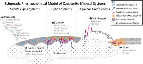
We thus provide a conceptual physicochemical model starting with a Sn-granite and classify cassiterite upon distinctions between mineral systems where cassiterite precipitates from a silicate liquid (Silicate Liquid Systems), those likely to be associated with precipitation from both silicate liquid and ore forming aqueous fluids (Hybrid Systems), and those in which cassiterite precipitates solely from ore forming aqueous fluids (Aqueous Fluid Systems). We provide a schematic outline of this model in Figure 1 and discuss each class below.

Figure 1. A schematic illustration of the physicochemical model of cassiterite mineral systems employed in this study. Silicate Liquid Systems, where cassiterite precipitates from a silicate liquid, include (a) pegmatite deposits, and (b) granite-hosted Disseminated Sn deposits. Hybrid Systems, where cassiterite may precipitate from both silicate liquids and aqueous fluids, are represented by (c) greisen deposits. Aqueous Fluid Systems, where cassiterite is precipitated from hydrothermal fluids only, are represented by (d) vein-hosted systems and (e) Sn-bearing skarn systems. In this model, the key distinction between vein-hosted and skarn systems is the degree of wall-rock alteration (metasomatism), with vein-hosted systems representing a low alteration endmember, and skarn systems representing a high alteration endmember. The classification of cassiterite crystals examined in this study is also listed in this figure.

Silicate liquid systems

The most economically significant deposits of this class are granitic pegmatites (Figure 1a), commonly of the Li–Cs–Ta (LCT) class (Černý & Ercit, 2005). Along with their Sn contents, they are generally enriched in other metals of economic interest such as Li, Cs, Ta and Nb. Although volatile saturation undoubtedly plays an important role in pegmatite crystallisation (London, 2014; Thomas & Davidson, 2016), the important characteristic for this type of mineral system in our physicochemical model is the silicate melt fraction of pegmatitic liquids; we do not classify or subdivide these systems further.

Cassiterite is also known to occur as disseminated crystals in Sn-granites (Figure 1b), either enclosed by, or intergrown with, magmatic minerals (feldspar, micas) and crystallise from magmas sufficiently enriched in Sn (e.g. Breiter et al., 2017). In both pegmatitic and granite-hosted systems, late-stage hydrothermal fluids may result in significant alteration of the host rock and produce post-primary growth modification structures in cassiterite, such as the CL-bright rehealed fractures observed in a cassiterite crystal from the granite-hosted White Lode deposit, Western Australia (Bennett et al., 2020). This local mobility of Sn was interpreted as the result of late-stage dissolution-reprecipitation processes.

Hybrid systems

It is well recognised that the aqueous fluids at the magmatic-hydrothermal transition may be capable of significant transport of Sn, primarily as a function of HCl activity (Duc-Tin et al., 2007; Heinrich, 1990; Hong et al., 2021; Schmidt, 2018; Vonopartis et al., 2020). If these fluids were unable to leave the host granite, they may have caused significant autometasomatic alteration (Černý et al., 2005; Piranjo, 2009), resulting in greisen systems (Figure 1c). In these systems, multiple paragenetic stages of cassiterite may be expected, such as an early comagmatic stage, a syn-ore hydrothermally precipitated stage from the greisen fluids, and a late alteration stage with local Sn-mobility. These different paragenetic stages may conceivably result in cassiterite crystals with contrasting chemistry, alternatively, they may form with distinct differences in internal chemical zonation. As such, cassiterite crystals from greisen systems may be expected to show ‘hybrid’ chemical characteristics of both Silicate Liquid System and Aqueous Fluid System endmembers.

Aqueous fluid systems

If the mineralising magmatic hydrothermal fluids escaped the host granite, they may have deposited Sn externally into the country rocks via cassiterite–quartz vein hosted or skarn systems (Benites et al., 2022; Černý et al., 2005; Hong et al., 2021; Meinert et al., 2005; Piranjo, 2009). In this model, we consider both systems as endmembers of a continuous series, primarily defined by the reactivity of the host rock. In other words, the main physicochemical distinctions here are the degree of wall-rock interaction, and the degree of mixing of the mineralising fluid with non-magmatic fluids, such as meteoric water.

In quartz vein hosted systems (Figure 1d), wall-rock interaction tends to be low and precipitation is driven by cooling and/or mixing with meteoric waters (Heinrich, 1990), i.e. the system is fluid-buffered. Quartz vein hosted systems emplaced within the parental granite (or other coeval magmatic rocks) without significant alteration are also within this class. Alternatively, if mineralising fluids escaped into a reactive host such as carbonate rocks, then cassiterite would precipitate as a result of metasomatic reactions (i.e. the system is rock-buffered), and skarn style mineralisation may result (Figure 1e).

Model caveats

The above classification scheme is intentionally simplistic, serving as a first-order framework for investigating the geochemical variability of cassiterite. Further details can discriminate mineral systems into more nuanced classifications. For example, we do not distinguish between different models for granite generation, depth of emplacement, subsequent volatile saturation, structural controls, or age-related diversity of Sn-mineral systems. In addition, some distinctive mineralisation styles have not been considered. These include the rhyolite-hosted Sn deposits of New Mexico (Lufkin, 1976, 1977) or cassiterite in volcanogenic massive sulfide (VMS) style deposits such as Neves-Corvo, Portugal (Serranti et al., 2002), for example.

This model also excludes cassiterite deposited from other precipitation mechanisms, such as generation via subsequent oxidation reactions of earlier stanniferous sulfosalts such as stannite (CuFeSnS₄), or precipitation via vapour condensation, known from some high temperature fumaroles on active volcanoes such as Iō-dake, Japan (Africano et al., 2014) and Tolbachik, Russia (Pekov et al., 2018). We instead leave further ‘splitting’ and subsequent refinement of our model to future studies with extended sample sets.

Methods

Samples

Cassiterite crystals from 18 localities (Table 2; Figure 1) were selected for this study to encompass the range of mineral systems identified in our physicochemical model: Sn-mineralised pegmatites (Poona Tin Shafts, Moolyella, Sifleetes Reward, Spear Hill, Trigg Hill, Bamboo Creek, Greenbushes, Emmons Pegmatite; Figure 1a), greisen systems (Buriti Mine, Pedra Branca, Blue Tier, Saltwater Creek; Figure 1c), hydrothermal cassiterite–quartz vein hosted systems (Aberfoyle, Elsmore; Figure 1d) and skarn systems (Mt Bischoff, Renison; Figure 1e). Disseminated Sn deposits (While Lode; Figure 1b) are represented in this study by a kaolinised coarse-grained granite, known as the ‘White Lode’, which contains disseminated primary magmatic cassiterite crystals and is spatially and temporally related to the Tin Shafts pegmatite at Poona. Due to a likely common paragenetic heritage, analyses from the White Lode cassiterite crystals are plotted with analyses of the Tin Shafts samples for comparison, alongside other pegmatite samples. Also included are alluvially collected cassiterite crystals from Beechworth with an unknown paragenesis. Generally, only one crystal from each locality was selected for analysis due to their large size (for instance, the crystal from Elsmore is ∼2 cm) with multiple transects targeting distinct sector zonation where identified. The exception are three small crystals from Mount Bischoff, analysed in situ within the same thin section. A summary of the general characteristics of each locality, and some key references, are also listed in Table 2, and images of each thin section and selected grain mount are included as a supplementary file (Appendix 1). Localities were primarily selected from Australia (in particular, Western Australia) due to the ready availability of samples to the authors of this study, and the general paucity of geochemical data previously published on Australian cassiterite crystals.

Table 2. Summary of the cassiterite samples and their localities used in this study, with approximate coordinates (accurate to within ±1 of the decimal place given). Each locality is classified into one of the simplified cassiterite mineral systems as outlined in Figure 1. Any coexisting mineral phases noted by previous authors are shown along with any classifications of each deposit type, for comparison (Paragenesis), taken from the key references for each locality. The nature of the samples used in this study, and any other notable characteristics, are described in Sample Observations and Characteristics.

Paragenesis/Locality (Latitude, Longitude)	References	Sample observations and characteristics
Granite-hosted disseminated Sn deposits
White Lode, Poona, Western Australia, Australia (–27.13°, 117.46°)
Kaolinised granite	Bennett et al., 2020; Grundmann & Morteani, 1998; Jacobson et al., 2007; Marshall et al., 2016	1–2 mm anhedral to euhedral cassiterite crystals disseminated in a kaolinite (after feldspar) quartz granitic matrix.
Pegmatite-hosted Sn deposits
Tin Shafts, Poona, Western Australia, Australia (–27.14°, 117.46°)
Lepidolite, cassiterite, columbite–tantalite, fluorite, garnet and apatite bearing pegmatite	Grundmann & Morteani, 1998; Jacobson et al., 2007; Marshall et al., 2016	∼5 mm anhedral crystal, collected loose from around the entrance to the shaft.
Moolyella, Western Australia, Australia (–21.14°, 119.89°)
Cassiterite, columbite–tantalite and magnetite bearing pegmatites	Jacobson et al., 2007	∼5 mm rounded eluvial crystal.
Sifleetes Reward, Western Australia, Australia (–21.27°, 118.61°)
Cassiterite, columbite, lepidolite, tourmaline and topaz bearing pegmatite	Jacobson et al., 2007	3 × 2 mm rectangular crystal in quartz–feldspar–mica pegmatitic matrix.
Spear Hill, Western Australia, Australia (–21.51°, 119.42°)
Cassiterite bearing pegmatites	Jacobson et al., 2007	∼10 mm sub-angular eluvial crystal.
Trigg Hill, Western Australia, Australia (–21.60°, 119.29°)
Cassiterite, monazite and tanteuxenite bearing microcline–quartz pegmatites	Jacobson et al., 2007; Sweetapple & Collins, 2002	2–3 mm rounded eluvial cassiterite crystals.
Greenbushes, Western Australia, Australia (–33.86°, 116.06°)
Cassiterite, tantalite, albite and spodumene bearing Sn–Ta–Li pegmatite	Partington et al., 1995	∼1 mm rounded eluvial crystal.
Bamboo Creek, Northern Territory, Australia (–13.07°, 130.71°)
Cassiterite, columbite–tantalite bearing muscovite–feldspar–quartz pegmatite	Ahmad, 1995; Summers, 1957	∼3 mm subangular crystal from mine tailings.
Emmons Pegmatite, Maine, USA (44.31°, –70.78°)
Cassiterite, columbite–tantalite, wodginite, tantalowodginite and phosphate bearing B–Li–Cs–Ta pegmatite	Falster et al., 2019	∼10 mm angular fragment, chipped off a blocky ∼30 mm crystal from a cassiterite–albite–quartz hand specimen.
Skarn-hosted Sn deposits
Mount Bischoff, Tasmania, Australia (–41.43°, 145.52°)
Cassiterite, quartz, pyrrhotite, pyrite, sellaite, fluorite and topaz skarn	Halley & Walshe, 1995; Walshe et al., 1996	Numerous equant crystals in thin section, with major quartz, sellaite, topaz, minor carbonates, clays, and trace pyrrhotite.
Renison Bell, Tasmania, Australia, (–41.80°, 145.44°)
Cassiterite, quartz, pyrrhotite, arsenopyrite and tourmaline skarn	Hutchinson, 1982; Walshe et al., 1996, 2011	∼300 µm cassiterite crystal protruding into a ∼400 µm cavity in massive cassiterite ore, with minor quartz
Deposits of unknown paragenesis
Beechworth, Victoria, Australia (–36.32, 146.67°)
Alluvial	Cochrane & Bowen, 1971; Dunn & Mahony, 1913	Numerous small (<1 mm) rounded alluvial cassiterite crystals.
Quartz vein-hosted Sn deposits
Aberfoyle, Tasmania, Australia (–41.65°, 147.75°)
Quartzite hosted muscovite, cassiterite, wolframite, quartz veins	Blissett, 1959	Comb-textured cassiterite crystals ∼ 1 cm long, radiating frosm a muscovite selvage. Trace chalcopyrite, sphalerite, galena as small inclusions in cassiterite.
Elsmore, New South Wales, Australia (–29.8°, 151.2°)
Cassiterite–quartz veins	Brown & Stroud, 1993	Large 2 cm lustrous black twinned cassiterite crystal, thin-sectioned perpendicular to the twin plane. From a private collection, exact location unknown.
Greisen-hosted Sn deposits
Blue Tier, Tasmania, Australia (–41.2°, 148.1°(?))
Cassiterite, quartz, muscovite and topaz greisen, with minor chalcopyrite, bornite, molybdenite and fluorite	Groves et al., 1977; Reid & Henderson, 1928	Large 1 cm lustrous black twinned cassiterite crystal, thin-sectioned perpendicular to the twin plane. From a private collection, assumed to be collected from the Anchor Mine.
Saltwater Creek, Tasmania, Australia (–42.11°, 148.27°)
Greisenised granite and quartz–cassiterite veins	Keid, 1951; Twelvetrees, 1901	Numerous small (<1 mm) rounded alluvial crystals.
Buriti Mine, Goiás, Brazil (–13.53°, –48.53°)
Hydrothermal albitite (Na-metasomatised granite)	Botelho & Moura, 1998; Lenharo et al., 2002	Numerous 1–2 mm angular crystals, supplied as a cassiterite concentrate.
Pedra Branca, Goiás, Brazil (–13.6°, –47.0°)
Cassiterite, topaz and Li-siderophyllite greisenised granite	Botelho & Moura, 1998; Lenharo et al., 2002	Numerous 1–2 mm angular crystals, supplied as a cassiterite concentrate.

EPMA transects

All analyses consist of transects across growth zones of cassiterite crystals revealed optically or via cathodoluminescence. The EPMA transects were acquired with the JEOL JXA-8530F Hyperprobe housed at the Centre for Microscopy, Characterisation and Analysis (CMCA) at the University of Western Australia (UWA). The transects were automatically generated between start and end points in the Probe for EPMA acquisition software (Donovan, 2018), with a 10 micrometre spacing. Points were then manually checked and adjusted as required to avoid inclusions or fractures visible under SEM imaging. When points were adjusted, a new position was selected perpendicular to the transect direction (i.e. along the same growth zone). We measured Sn, Ti, Fe, Mn, Nb, Ta, Zr and W, along with Na, Al, Si and Ca for inclusion detection, using a fully focused electron beam at 20 kV and 80 nA. The analysis routine is listed in Table 3, along with the standards used for calibration. The data were processed using the Probe for EPMA software package (Donovan, 2018).

Table 3. EPMA acquisition routine for the cassiterite crystals analysed in this study.

Element/Line	Crystal	Count time (s)	Standard
Sn Lα	PETJ	40	Cassiterite
Ti Kα	PETJ	50	Rutile
Fe Kα	LiF	40	Magnetite
Mn Kα	LiF	40	Mn
W Lα	LiF	40	Scheelite
Ta Lα	LiF	50	Manganotantalite
Nb Lα	PETH	40	CaNb2O6
Zr Lα	PETH	60	Zr
Si Kα	TAP	20	Jadeite
Al Kα	TAP	40	Corundum
Na Kα	TAP	40	Jadeite
Ca Kα	PETH	40	Fluorite

Data analysis

Following initial data processing in Probe for EPMA (mean atomic background correction, interference calculations), the results of each analysis were exported from Probe for EPMA to a .csv file and further processed in the R programming language. The data from each transect were manually curated to remove any analyses where surface contamination (from the occasional dust grain that had adhered to the surface post carbon coating) or subsurface inclusions may have impacted the results. These may manifest as abnormally low or high elemental totals, or as low Sn contents. Analyses were also rejected for high Na, Al, Si or Ca contents outside the range for the majority of the transect, which for these elements is generally below the background. The original exported .csv files (organised by date), the R processing code (which includes comments on why individual points were excluded), and the final organised dataset are available in the GitHub repository, and the final organised dataset is also included as an online supplementary file.

The plots in each figure were also generated in the R programming language, using the ggplot2 (Wickham, 2016) and ggtern (Hamilton, 2017) packages. For the final preparation of the figures presented in this paper, these plots were then exported to a vector graphic software package for minor aesthetic touches (such as compilation of sub-plots into one figure, addition of annotations or labels where needed). However, the R codes for the reproduction of the basic plots within each figure are also available online in the GitHub repository.

Theoretical framework

Our approach in this contribution towards understanding the uptake of minor elements into the cassiterite lattice begins with a list of charge-balanced substitution mechanisms, in which all theoretically possible stoichiometries of M⁶⁺, M⁵⁺, M⁴⁺, M³⁺ and M²⁺ cations are included, without prior bias on the applicability of uncommon or unobserved redox states. We then also compile a table of hypothetical endmembers for the limited solid solution series using crystallographic data from natural and synthetic mineral analogues. Both of these tables are presented in the discussion and serve as a framework for our interpretation of the EPMA data presented in this study.

Oxygen fugacity speciation curves

Some of the substitution mechanisms considered in our theoretical framework involve uncommon, or unexpected, oxidation states. As an independent constraint on the applicability of these substitutions, simple metal-oxide oxygen fugacity buffers were generated from first principles of thermodynamics, using data obtained from NIST-JANAF thermochemical tables (Allison, 2013) where available, and from individual literature sources if not included in NIST-JANAF. The specific source for each chemical component is listed in the data file included in the GitHub repository (thermodynamic_data.xlsx). The buffer equations were calculated and plotted in R. The standard suite of geochemical f_O2 reference buffer curves (listed in Table 4) from iron–wüstite (IW) to magnetite–hematite (MH) were reproduced from first principles, using the NIST-JANAF data, for comparison with the non-standard oxides in consideration (such as WO₂–WO₃). These serve not only as a reference to more familiar buffers, but also as a sanity check on the validity of the calculations.

Table 4. Oxygen fugacity reactions considered in this study. Buffer curves calculated from these equations are displayed in Figure 4. The typical buffer series of Magnetite–Hematite (MH), Nickel–Nickel Oxide (NNO), Fayalite–Magnetite–Quartz (FMQ), Wüstite–Magnetite (WM), Iron–Wüstite (IW), and Quartz–Iron–Fayalite (QIF) were also calculated and displayed for comparison.

Abbreviation	Reaction
MH	4Fe3O4 + O2 ⇌ 6Fe2O3
NNO	2Ni + O2 ⇌ 2NiO
FMQ	3Fe2SiO4 + O2 ⇌ 3SiO2 + 2Fe3O4
WM	6FeO + O2 ⇌ 2Fe3O4
IW	2Fe + O2 ⇌ 2FeO
QIF	SiO2 + 2Fe + O2 ⇌ 2Fe2SiO4
WO2:WO3	2WO2 + O2 ⇌ 2WO3
Sn:SnO2	Sn + O2 ⇌ SnO2
H2:H2O	2H2 + O2 ⇌ 2H2O
CH4:CO2	½CH4 + O2 ⇌ ½CO2 + 2H2O
NbO2:Nb2O5	4NbO2 + O2 ⇌ 2Nb2O5
Ta:Ta2O5	4/5 Ta + O2 ⇌ 2/5 Ta2O5

Available thermodynamic data for the reactions Sn + ½O₂ ⇌ Sn²⁺O and Sn²⁺O + ½O₂ ⇌ Sn⁴⁺O₂ provide inconsistent calculations with the data for Sn + O₂ ⇌ Sn⁴⁺O₂. This is probably due to experimental difficulties limiting the oxidation of Sn to SnO. As these buffer curves represent the equal activities (i.e. mid-points) of the oxides on each side of the oxidation reaction, the reaction curve for SnO–SnO₂ is sufficiently constrained within the region of the Sn–SnO₂ reaction. Hence, we employ the Sn–SnO₂ curve as a general proxy for SnO–SnO₂.

Speciation curves for each of these reactions were also generated to compare the relative proportions of oxide species within the expected f_O2 range of cassiterite mineral systems, following the methodology of Matjuschkin et al. (2016) and outlined in the supplementary R file in the Github repository. These are a first-order approximation, modelled as a general silicate melt or hydrothermal fluid, in order to provide a starting scaffold to guide further studies and detailed thermodynamic considerations where highlighted by the results of this contribution.

Lattice strain model

A lattice strain model for estimation of partitioning behaviour was also developed in R following the equations of Blundy and Wood (1994, 2003) and Wood and Blundy (2001). In the original lattice strain model, the modelled partition coefficients are constrained by some known coefficients between the mineral and growth medium of interest, i.e. the incorporation of known coefficients is what determines the nature of the parental composition. In the absence of any measured partition coefficients for minor elements in naturally occurring cassiterite, or in any experimentally derived analogues, we here use a partition coefficient for a given minor element (Mⁿ⁺) between cassiterite (cst) and an undefined hypothetical liquid (liq), normalised to a hypothetical Sn⁴⁺ partition coefficient of D₀₀ = 1, using the ionic radius of Sn⁴⁺ in VI-fold coordination as an approximation for the size of the lattice site (r_i = 0.69; Shannon & Prewitt, 1969). In this manner, the partition coefficient ^cst/liqD_M/Sn (abbreviated to D’ and referred to as a ‘relative partition coefficient’) represents the theoretical lattice strain due to size and charge differences, expressed as a relative magnitude of whatever the actual partition coefficient between cassiterite and the host liquid may be. It is important to note that this model does not distinguish between a silicate magma or an aqueous fluid, as we have no measured partition coefficients for elements between cassiterite and silicate or aqueous liquids with which to anchor our model. We estimate Youngs elastic modulus (E) for cassiterite derived from measurements for the shear elastic modulus (G) and bulk elastic modulus (K) (Chang & Graham, 1975), and assuming isotropic behaviour (even though cassiterite is tetragonal, and this is not the case). Thus, our model only considers partitioning during crystallisation from a generalised parental liquid, is not reflective of any real partition coefficients, and should not be used to calculate any real partition coefficients in the future. As with the oxygen fugacity speciation modelling, this is intended only as a first-order approximation to aid in the interpretation of the results of this paper. This model should be viewed as a simple, but useful tool, with values close to 1 indicative of highly compatible behaviour, and values much less than 1 indicative of highly incompatible behaviour.

Results

General summary and statistics of EPMA analyses

A set of summary statistics for each of the cassiterite crystals studied are provided as supplementary files in the GitHub repository, in weight percent (wt%), atomic percent (at%) and atoms per formula unit, times 100 (apfu*100). For convenience, all further discussion is based on the data presented as either at% or apfu*100. These statistics are best presented graphically through a series of box plots. However, the cassiterite crystals examined in this study show oscillatory and sector zonation, even in crystals where primary growth structures are obscured by a dark CL response. Thus, although box plots are sufficient to describe the asymmetry of normal distributions, they fail where the data are multi-modal due to the intracrystalline variability of these samples. This variability is instead best visualised through violin plots, which are symmetrically presented probability density curves. These violins are then easily compared with one another, allowing for observations of intracrystalline variability within, and intercrystalline variability between the samples.

In Figures 2 and 3, the length of the violins along the x-axis shows the range of compositions (in atomic percent along the bottom, in apfu*100 across the top) for each locality represented on the y-axis. The thickness of the violins along the y-axis corresponds to the normalised probability density, i.e. the modes of each sample have been normalised to the same thickness to account for differing sample sizes. The violins are also not calculated beyond the minimum and maximum extents of the data. This has a combined effect that results in sharp vertical cuts (such as observed for the lower limit of Sn at Emmons; Figure 2a) in samples with lower total analyses where values sufficiently low or high enough to ‘close-off’ the violins were not encountered. All analyses were included in the density distribution, with those below detection set to zero. This allows the shape of the violins at concentrations just above the lower limit of detection (LLD) to truly reflect the distribution of analyses at this concentration. The extents of the x-axes are chosen to allow visual comparison between compositions of adjacent panels (most are set to a maximum of 1.5 at%), rather than to fill the plot. For Zr and Mn (extents of 0.25 at%; Figures 2c and 3c) and W (an extent of 0.6 at%; Figure 2d), the scales were chosen to highlight the variability between samples without visually dominating the figure. The violins for each locality are grouped along the y-axis according to the dominant mineralisation environment (as outlined in Figure 1), with the exception of Beechworth, which has an unknown paragenesis due to its alluvial nature.

Figure 2. Intracrystalline and intercrystalline variability of substitutional elements in the cassiterite crystals analysed in this study, presented as violin plots in at% (bottom x-axis) and apfu*100 (top x-axis). See text for discussion. One-sigma uncertainty (σ) is numerically labelled on the bottom x-axis for each element, and the two-sigma uncertainty (2σ) is shown graphically as an error bar inset in each plot. (a) Variability in total Sn concentration. The total number of analyses (n), mean (orange circle) and median (vertical blue line) values are highlighted in the key. The dashed black line represents the stoichiometric ideal. (b) Variability in Ti. The lower limit of detection (LLD), the number of analyses below this threshold (n < LLD) and the number above (n > LLD) are highlighted in the key along with the mean and median and are used throughout the rest of the figure. (c) Variability in Zr. (d) Variability in W.

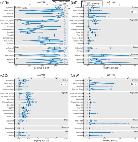
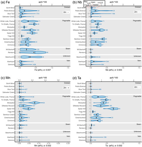
Figure 3. Intracrystalline and intercrystalline variability of substitutional elements in the cassiterite crystals analysed in this study, presented as violin plots in at% (bottom x-axis) and apfu*100 (top x-axis). Continued from Figure 2. (a) Variability in Fe. (b) Variability in Nb. (c) Variability in Mn. (d) Variability in Ta.

The range in total Sn contents shows that there is no clear contrast in the mean or median scores between different mineralisation styles, although a general trend in pegmatitic cassiterite towards lower concentrations (less stoichiometrically pure cassiterite) can be observed (Figure 2a). Bimodality is clearly displayed in some samples (e.g. Buriti Mine, Blue Tier, White Lode, Emmons), whereas others display more subtle bimodal distributions (e.g. Tin Shafts, Sifleetes Reward, Bamboo Creek) and some display normal distributions (e.g. Saltwater Creek, Elsmore). In Figure 2b, only cassiterite from Buriti Mine and White Lode show bimodal Ti distributions. Cassiterite from hydrothermal vein systems shows the highest concentrations of Ti in general. No Ti was measured above the LLD in the Emmons cassiterite sample.

The Zr concentrations are generally low with near symmetric normal distributions, with the bulk of analyses within ±2σ of the mean (Figure 2c). A subordinate mode is observed in the tails leading towards values lower than the mean in both the White Lode and Sifleetes Reward samples. The Pedra Branca sample is unique in that the subordinate mode is located at higher concentrations than the mean. The highest concentrations of Zr are observed in the pegmatitic cassiterite crystals. The mean for Saltwater Creek appears to be centred on the LLD (a near equal number of analyses above and below this threshold), whereas the means for Renison and Beechworth are clearly below the LLD.

Only a few localities show substitutional W to any measurable degree (Figure 2d). Pedra Branca, Saltwater Creek and Renison show the highest mean W concentrations, which appear to correlate with a high number of analyses above the LLD relative to the number of analyses below the LLD. The total range is similar for these localities, along with Blue Tier, Aberfoyle and Elsmore. Only Sifleetes Reward and Mount Bischoff show values entirely above the LLD, and both are unimodal. There are a few analyses of W concentrations above the LLD for each of the Buriti, Bamboo Creek, Greenbushes, Emmons and Beechworth samples; W was not detected in the remaining samples.

Similar distributions are seen between Fe (Figure 3a), Nb (Figure 3b), Mn (Figure 3c) and Ta (Figure 3d). The overall shape of the violins shows particularly similar distributions between Fe and Nb for all samples except for the Mount Bischoff, Renison, and Beechworth samples, which show some of the highest Fe concentrations, but Nb (as well as Ta and Mn) concentrations below or within ±2σ of the LLD. Manganese is detectable in most samples; however, the mean values lie below the LLD for all samples except for cassiterite crystals from pegmatitic environments. The pegmatitic samples also show Ta concentrations comparable to Nb, with a few samples showing higher Ta than Nb, in particular Spear Hill. The non-pegmatitic samples show measurable, but comparatively insignificant, Ta concentrations.

Theoretical models

Oxygen fugacity speciation curves

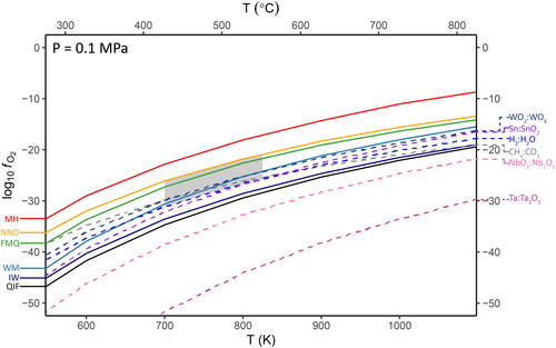
The calculated f_O2 buffer curves for the reactions listed in Table 4 are shown in Figure 4. The lower bound in the expected range of f_O2 for cassiterite mineralising systems (grey region) was calculated as the stability of water via the H₂:H₂O reaction, whereas the upper bound was constrained to the NNO buffer due to the typically reduced nature of these systems (Bhalla et al., 2005; Ishihara, 1979; Linnen et al., 1995; Taylor, 1979). At temperatures below 850 K (≃577 °C, a typical upper limit for Sn mineralisation; Heinrich, 1990), the WO₂:WO₃, H₂:H₂O and CH₄:CO₂ buffer curves lie at higher f_O2 than the Sn:SnO₂ buffer, while the NbO₂:Nb₂O₅ and Ta:Ta₂O₅ buffer curves are well below the QIF buffer.

Figure 4. Oxygen fugacity buffer curves for the standard set (QIF to MH, left) with the reactions of interest to this study (right). The grey area represents the expected f_O2 of most cassiterite mineral systems (Bhalla et al., 2005; Ishihara, 1979; Linnen et al., 1995) and an expected upper T range of primary Sn-mineralising fluids in these systems (Heinrich, 1990).

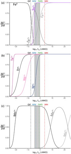
The speciation curves generated using these buffer equations show that in cassiterite mineralising systems the dominant species for Fe is expected to be Fe²⁺, with increasing Fe³⁺ towards higher f_O2 (Figure 5a). A minor amount of Nb⁴⁺ is likely to be present, particularly towards the lower limits of the expected cassiterite-mineralising region, whereas the model predicts that W is likely to switch from a W⁴⁺ dominant to a W⁶⁺ dominant regime, approximately coincident with the WM buffer at the modelled temperature of 800 K (Figure 5b). Both Ta and Ti are modelled to be almost entirely in their highest oxidation states at these conditions. Only the Mn²⁺ state is modelled to be present at these conditions (Figure 5c).

Figure 5. Oxygen fugacity speciation curves for oxidation states of interest, calculated at 800 K. The overall geometry of these curves is similar at lower temperatures. The grey area shows the projected range in f_O2 from Figure 4. The mid-points (equal activities) of the QIF, WM, QFM and MH buffers are shown as dashed vertical lines, using the same colour scheme as Figure 4. (a) The magenta line displays the total proportion of Sn⁴⁺ as a function of f_O2 for the Sn:SnO₂ reaction, the black to grey lines display the total proportion of Fe species. (b) The dark pink line displays the total proportion of Ta⁵⁺ for the Ta:Ta₂O₅ equation, the light pink line the proportion of Nb⁵⁺ for the NbO₂:Nb₂O₅ equation. The blue line is the total proportion of W⁶⁺ for the WO₂:WO₃ equation, and black line is the total proportion of Ti⁴⁺ over the proportion of Ti³⁺. (c) The black to grey lines display the changing speciation of Mn species.

Lattice strain model

The lattice strain model predicts that Nb, W, Zr and Ti have a strong affinity for the cassiterite lattice in their tetravalent states, with relative partition coefficients an order of magnitude higher than pentavalent Nb, Ta and W and trivalent Fe and Mn (Figure 6a). Hexavalent W, and divalent Fe and Mn are predicted to show relative partition coefficients four orders of magnitude lower than Sn⁴⁺. However, as these elements are incorporated via charge balanced coupled substitutions, the strain related to charge difference is nullified. In Figure 6b, the potential charge balanced coupled substitution mechanisms are compared with the single ionic substitutions, using a stoichiometrically averaged ionic radius to model the net lattice strain experienced due to size mismatch. In this model, the coupled substitution of columbite/tantalite–(Fe) stoichiometry (Equations 14 and 15; Table 5) has an identical averaged ionic radius to Sn⁴⁺, and thus an identical relative partition coefficient. This is closely followed by the ferberite stoichiometry (Equation 20; Table 5) and the hypothetical 2 W⁵⁺Mn²⁺ substitution (Equation 19; Table 5). The remaining coupled substitution mechanisms all have relative partition coefficients higher than that predicted for Ti⁴⁺.

Figure 6. Lattice strain model for the possible substitution mechanisms of minor elements in cassiterite. (a) Predicted partition coefficients for ions only, including strain due to charge mismatch. (b) Partition coefficients using stoichiometrically averaged ionic radii (i.e. the ionic radius for the substitution of 2Nb⁵⁺Fe²⁺ is modelled as [2r_Nb5++r_Fe2+]/3). Charge is balanced in this instance, so strain only results from the combined radii mismatch. Note that the combination of larger and smaller cations results in an overall effective ionic radius similar to Sn⁴⁺.

Table 5. Possible substitution mechanisms for minor element incorporation into cassiterite. The different mechanisms are grouped into classes defined by the highest valency in the substitution reaction. The stoichiometric coupling reflects the ratio between cations in coupled substitutional pairs. The equations show the full substitution replacement reactions with Sn⁴⁺ into the cassiterite lattice. Each reaction has an assigned number, which will be used throughout the text. The ionic radius in six-fold (octahedral) coordination (Shannon & Prewitt, 1969) is shown for each cation (in Angstroms, Å), along with the radius for Sn⁴⁺ for comparison. Where the reaction contains multiple cations, the ionic radius shown is the stoichiometrically averaged radius for that reaction. An asterisk (*) denotes substitution reactions disregarded or not considered in previous literature.

Class, Coupling
	Equation (Eq. #)	IR^(VI) (Å)
Trivalent, Uncoupled
Fe^3+ + 1/3 Fei^3+ ⇌ Sn^4+ + □i	(1)	0.645
Fe^3+ + OH^– ⇌ Sn^4+ + O^2–	(2)	0.645
Tetravalent, Uncoupled
Si^4+ ⇌ Sn^4+	(3)	0.400
Mn^4+⇌ Sn^4+	(4)*	0.530
Ti^4+⇌ Sn^4+	(5)	0.605
W^4+⇌ Sn^4+	(6)	0.660
Nb^4+⇌ Sn^4+	(7)	0.680
Ta^4+⇌ Sn^4+	(8)	0.680
Sn^4+		0.690
Zr^4+⇌ Sn^4+	(9)	0.720
Pentavalent, 1:1
Nb^5+ + Fe^3+ ⇌ 2Sn^4+	(10)	0.643
Ta^5+ + Fe^3+ ⇌ 2Sn^4+	(11)	0.643
Nb^5+ + Mn^3+ ⇌ 2Sn^4+	(12)	0.643
Ta^5+ + Mn^3+ ⇌ 2Sn^4+	(13)	0.643
Pentavalent, 2:1
2Nb^5+ + Fe^2+ ⇌ 3Sn^4+	(14)	0.687
2Ta^5+ + Mn^2+ ⇌ 3Sn^4+	(15)	0.687
2Nb^5+ + Fe^2+ ⇌ 3Sn^4+	(16)	0.703
2Ta^5+ + Mn^2+ ⇌ 3Sn^4+	(17)	0.703
2W^5+ + Fe^2+ ⇌ 3Sn^4+	(18)*	0.673
2W^5+ + Mn^2+ ⇌ 3Sn^4+	(19)*	0.690
Hexavalent, 1:1
W^6+ + Fe^2+ ⇌ 2Sn^4+	(20)	0.690
W^6+ + Mn^2+ ⇌ 2Sn^4+	(21)*	0.635
Hexavalent, 1:2
W^6+ + 2Fe^3+ ⇌ 3Sn^4+	(22)	0.630
W^6+ + 2Mn^3+ ⇌ 3Sn^4+	(23)*	0.587

Discussion

We divide our discussion into two parts. In the first section, we compare our EPMA results with a list of proposed substitution mechanisms and discuss these data in light of our oxygen fugacity and lattice strain models. In the second section, we use the insights gained from the first section to discuss the applied use of minor element substitution variability in cassiterite towards the development of a paragenetic classification diagram. These observations are then used to provide a constraint on the primary source of the Beechworth alluvial cassiterite.

Substitution mechanisms

A list of substitution reactions considered in this contribution are outlined and numbered in Table 5, with any corresponding references and prior evidence for their existence summarised in Table 6. The possible charge balanced substitutions that have not been previously considered in the literature may be due to either a lack of evidence, or due to oxidation states considered outside the expected range in f_O2 of Sn-mineralising systems. These reactions are marked by an asterisk in Table 5. They are included here for completeness, and for comparison with the results of our oxygen fugacity speciation curves in Figure 5.

Table 6. Existing evidence for the substitution mechanisms outlined in Table 5. Each cell contains a tick (✓) if the evidence is in favour of the substitution mechanism, a cross (×) if the evidence does not support this mechanism, and a question mark (?) if the evidence is ambiguous or uncertain. The analytical methods are also described in each cell, as one of stoichiometric analysis via electron probe microanalysis (EPMA), direct measurement of oxidation states via electron paramagnetic resonance (EPR) or Mössbauer Spectroscopy (Möss), or consideration of the local electronic environment via cathodoluminescence theory (CL). Direct measurement of OH content by Fourier Transform Infrared spectroscopy (FTIR) is also included.

	Reference	a	b	c	d	e	f	g	h	i	j	k	l
(Eq.#)	Equation
(1)	Fe^3+ + 1/3 Fei^3+		✓EPR					×EPMA			×EPMA	×EPMA
(2)	Fe^3+ + OH^-			✓EPR	✓Möss	✓EPR	? EPMA	×EPMA	✓FTIR	✓FTIR	×EPMA	×EPMA	? EPMA
(3)	Si^4+	✓CL
(5)	Ti^4+	✓CL	✓EPR			✓EPR	✓EPMA	✓EPMA			✓EPMA		✓EPMA
(6)	W^4+	? CL			? EPMA						×EPMA
(7)	Nb^4+				? EPMA						×EPMA
(8)	Ta^4+				? EPMA						×EPMA
(9)	Zr^4+							✓EPMA			✓EPMA
(10)	Nb^5+ + Fe^3+	? CL	✓EPR	✓EPR	× Möss	✓EPR	? EPMA	×EPMA			×EPMA	×EPMA	? EPMA
(11)	Ta^5+ + Fe^3+	? CL	✓EPR		× Möss		? EPMA	×EPMA			×EPMA	×EPMA	? EPMA
(12)	Nb^5+ + Mn^3+				× Möss		? EPMA	×EPMA			×EPMA	×EPMA	? EPMA
(13)	Ta^5+ + Mn^3+				× Möss		? EPMA	×EPMA			×EPMA	×EPMA	? EPMA
(14)	2Nb^5+ + Fe^2+	? CL			✓EPMA		✓EPMA	✓EPMA			✓EPMA	✓EPMA	✓EPMA
(15)	2Ta^5+ + Mn^2+	? CL			✓EPMA		✓EPMA	✓EPMA			✓EPMA	✓EPMA	✓EPMA
(16)	2Nb^5+ + Fe^2+				✓EPMA		✓EPMA	✓EPMA			✓EPMA	✓EPMA	✓EPMA
(17)	2Ta^5+ + Mn^2+				✓EPMA		✓EPMA	✓EPMA			✓EPMA	✓EPMA	✓EPMA
(20)	W^6+ + Fe^2+	? CL			×EPMA						? EPMA
(22)	W^6+ + 2Fe^3+	?CL			✓EPMA

a, Hall & Ribbe (1971); b, Izoret et al. (1985); c, Dusausoy et al. (1988); d, Möller et al. (1988); e, Ruck et al. (1989); f, Neiva (1996); g, Masau et al. (2000); h, Maldener et al., 2001; I, Losos & Beran (2004); j, Černý et al. (2004); k, Pal et al. (2007); l, Neiva (2008).

The substitution of minor elements into cassiterite may be considered as products of very limited solid solution series with hypothetical end-member mineral phases. These potential solid solution candidates are summarised in Table 7. This theoretical framework differs slightly from the ionic charge and size constraints considered in the lattice strain modelling, in that it allows comparison of crystallographic differences. Solid solution series are more likely to occur between two phases that share the same structure, such as forsterite–fayalite and enstatite–ferrosilite. However, solubility is very limited between phases where cationic substitutions appear to be straightforward, but there is a mismatch of crystal structures. A good example is the exchange of Si⁴⁺ ⇌ Ti⁴⁺ between quartz (SiO₂) and rutile (TiO₂), where the cations exist under a fourfold tetrahedral coordination in trigonal quartz, but a sixfold octahedral coordination in tetragonal rutile (Thomas et al., 2010).

Table 7. Possible end-member phases for (limited) solid solution series with cassiterite, corresponding to the substitution mechanisms in Table 5 (listed under Eq.#). The class (Tet., Tetragonal; Orth., Orthorhombic; Mon., Monoclinic; Trig., Trigonal), symmetry (space group) and unit cell parameters (lengths in Å, angles in degrees) for each phase are also listed. Data sourced from mindat.org (accessed 5th April 2020), except where referenced. Phases synthesised in a laboratory, and not known in nature, are labelled as synthetic.

Phase	Formula	Eq. #	Class	Symmetry	a	b	c	β
Rutile group
Cassiterite^a	SnO2	–	Tet.	P42/mnm	4.7382(4)		3.1871(1)
Stishovite^a	SiO2	3	Tet.	P42/mnm	4.1790(4)		2.6649(4)
Pyrolusite^a	MnO2	4	Tet.	P42/mnm	4.3980(1)		2.8726(1)
Rutile^a,b	TiO2	5	Tet.	P42/mnm	4.5937(1)		2.9587(1)
Synthetic^c	NbO2	7	Tet.	P42/mnm	4.8464(1)		3.0316(1)
Synthetic^d	TaO2	8	Tet.	P42/mnm	4.709		3.065
Other M^4+O2
Quartz	SiO2	3	Trig.	P3121	4.9133		5.4053
α-Cristobalite	SiO2	3	Tet.	P41212	4.9709(1)		6.9278(2)
Anatase	TiO2	5	Tet.	I41/amd	3.7845		9.5143
Synthetic^e	WO2	6	Mon.	P21/c	5.650(5)	4.892(5)	5.550(5)	120.42(7)
Baddeleyite^f	ZrO2	9	Mon.	P21/b	5.1505	5.2116	5.3173	99.23
Zircon	ZrSiO4	3,9	Tet.	I41/amd	6.607(1)		5.982(1)
Columbite group^g
Tapiolite	Fe^2+Ta2O6	15	Tet.	P42/mnm	4.762		9.272
Tantalite-(Fe)	Fe^2+Ta2O6	15	Orth.	Pbcn	5.73	14.24	5.08
Tantalite-(Mn)	Mn^2+Ta2O6	17	Orth.	Pbcn	5.7661(8)	14.44	5.093
Columbite-(Fe)	Fe^2+Nb2O6	14	Orth.	Pbcn	5.7321(4)	14.266(1)	5.0503(4)
Columbite-(Mn)	Mn^2+Nb2O6	16	Orth.	Pbcn	5.7637(7)	14.433(2)	5.0832(8)
Excess M^3+
Hematite	Fe2O3	1	Trig.	R-3c	5.038(2)		13.772(12)
Goethite	α-FeO(OH)	2	Orth.	Pnma	4.608	9.956	3.0215
Varlamoffite^h	(Sn,Fe)(O,OH)2	2	– Not formally described –
Wolframite group
Ferberite	Fe^2+WO4	20	Mon.	P2/b	4.72	5.7	4.96	90
Hübnerite	Mn^2+WO4	21	Mon.	P2/b	4.8238(7)	5.7504(10)	4.9901(8)	91.18(1)

^aBolzan et al., 1997, references therein. ^bNaidu & Virkar, 1998 report up to 7 ± 4 mol% TiO₂ in synthetic SnO₂. ^cDisplays the dirutile structure, but with tetragonal symmetry (Rogers et al., 1969). ^dSchönberg et al., 1954 report probable continuous solid solution between TaO₂ and TiO₂, but limited solid solution with VO₂ (which has a modulated dirutile structure). ^eMagnéli et al., 1952. Structurally very similar to rutile (dirutile structure), the WO₆ octahedra are slightly more deformed and drawn together into doublets due to metal-metal bonds (Magnéli et al., 1955). ^fDhage et al., 2006 report up to 25 mol% ZrO₂ in synthetic SnO₂. ^gThe columbite group minerals display solid solution and a variable degree of cation order, resulting in a wide range of unit cell parameters (Ercit et al., 1995). A miscibility gap exists between the tapiolite structure and that of columbite-tantalite (Černý et al., 1992). ^hAn International Mineralogical Association (IMA) approved but ‘questionable’ species, yet to be formally described due to the lack of sufficiently sized crystals for proper analysis (Jambor et al., 1995; Sharko, 1971).

In Table 5, we organise and classify these reactions by defining four families of substitution reactions based on the highest valence state of the substituting cation, here named the ‘Trivalent’, ‘Tetravalent’, ‘Pentavalent’ and ‘Hexavalent’ classes. The Pentavalent and Hexavalent classes have been further subdivided based on the stoichiometry of the coupled substitutions into the ‘2:1’, ‘1:1’ and ‘1:2’ subclasses. In our following discussion, we use the notation of M^p+ and Xⁿ⁺, where M is the metal with the highest valence of p+, and X is the charge balancing cation (with lower valence of n+) in coupled substitutional pairs. We will consider each reaction listed in Table 5 in order, below.

Trivalent class

Most of the existing discussion for this class is focused on the incorporation of Fe³⁺ without Nb, Ta or W, and has previously been termed as ‘excess Fe’ reactions by Izoret et al. (1985). There are two previously proposed mechanisms whereby charge is balanced in this case.

Equation 1: In the first mechanism, Fe³⁺ achieves charge balance with a component of Fe³⁺ in an interstitial lattice position. In this model, charge is balanced only if one-third of these interstitial sites are filled (i.e. only one interstitial Fe³⁺ is required for every three Fe³⁺ in the octahedral site). Izoret et al. (1985) suggest that the interstitial sites are generated via a coexisting substitution of Ti, which provides enough adjacent space due to the smaller ionic radius (0.605 Å for Ti⁴⁺ vs 0.690 Å for Sn⁴⁺; Shannon, 1976).

Such a correlation between an excess of Fe and Ti observed by Izoret et al. (1985) was not observed in any sample of this study. In particular, the Renison cassiterite sample, which contains the highest Fe concentrations observed (Figure 3a), contains almost no Ti (Figure 2b). Along with the sample from Mount Bischoff, they also show little to no Nb (Figure 3b) or Ta (Figure 3d), ruling out the incorporation of Fe via Fe–Nb–Ta coupled substitution mechanisms in these samples, but they do contain W (Figure 2d). In Figure 7, analyses plotting along the x-axis represent substitution of Fe without W, as is observed with all analyses from Mount Bischoff, and about half of those from Renison (Figure 7d). The excess Fe in these samples can only be explained by an Fe-only substitution mechanism (i.e. not coupled with any other metal cations). With no correlating Ti, the mechanism of Equation 1 appears to be unlikely to play any significant role in the samples presented in this study.

Figure 7. Binary plot of the substitutional relationship between Fe + Mn and W. The grey trend lines represent stoichiometries of 1:2 for Equations 22 and 23, 1:1 for Equations 20 and 21, and 2:1 for Equations 18 and 19. Points plotting in regions defined between these lines require a component of each bounding substitutional stoichiometry. Samples are grouped according to (a) pegmatitic and granite-hosted systems, (b) greisen systems, (c) vein-hosted systems, and (d) skarn systems. Note that the horizontal trend along the x-axis observed for Sifleetes Reward (in A) is due to the substitution of Fe coupled with Nb and Ta.

Equation 2: In the second mechanism, the presence of Fe³⁺ is balanced via the protonation of one oxygen to form an OH^- complex. This is the mechanism most favoured in prior studies (Table 1). Further evidence for a substitution of this type has also been observed in other rutile structure group minerals (Swope et al., 1995), and this substitution probably represents a limited solid solution series with varlamoffite (Table 7), a poorly described species due to the lack of suitable crystals for proper analysis (Jambor et al., 1995; Sharko, 1971).

Confirmation of this substitution mechanism in the cassiterite of this study cannot be ascertained further with EPMA data alone, however we consider that Equation 2 is likely the dominant mechanism for the incorporation of ‘excess iron’. As this mechanism involves OH^– or H⁺, depending on how the equation is written, it is likely pH sensitive; further investigation of this mechanism may prove it to be a useful indicator of fluid chemistry in Sn-bearing hydrothermal mineral systems.

Tetravalent class

These reactions do not require charge balance; as a result, direct substitution of M⁴⁺ cations into the cassiterite lattice is possible.

Equation 3: The substitution of Si⁴⁺ appears to be a straightforward homovalent substitution. However, the results of the lattice strain model predict that Si is too small in ionic radius to substitute for Sn⁴⁺ to any degree quantifiable by EPMA (Figure 6), in agreement with our observations. Furthermore, while stishovite (SiO₂) is a member of the rutile structure group (Table 7), it is an ultrahigh pressure (>16 GPa) phase first reported in an impact crater (Chao et al., 1962). The (SiO₂) polymorphs at more relevant pressure and temperature conditions are quartz and cristobalite (Table 7). Neither of these have structures similar to cassiterite, providing a further explanation for the lack of Si observed in the cassiterite of this study. Previous analyses of Si in cassiterite by Hall and Ribbe (1971) and Moore and Howie (1979) were performed by Energy Dispersive X-ray Spectroscopy (EDS) and are likely due to misidentification errors or poor interference calculations. The Si Kα lines (Kα₁ = 1.739 keV, Kα₂ = 1.741 keV; Deslattes et al., 2003) are centred between the Ta Mα and Ta Mβ lines: this is a known ‘problem region’ for peak identification of minor components (Newbury, 2009).

Monte Carlo simulated characteristic X-ray spectra generated using the NIST DTSA-II software package (Ritchie, 2009, 2019) for cassiterite doped with minor amounts of Ta and Si (1 apfu*100) are compared in Figure 8. In this simulation, the observed peaks for the Ta Mα and Mβ lines merge into one peak, the centre of which is indistinguishable from Si Kα. It is clear that at low Ta concentrations, even such as those seen in hydrothermal vein cassiterite crystals (such as Aberfoyle, with a mean Ta content of 0.069 apfu*100 and maximum of 1.21 apfu*100), spurious Si values may be assumed if the peaks are not recognised as Ta M lines.

Figure 8. Monte Carlo simulation of a pure cassiterite EDS spectrum (black line), compared with simulated spectra of cassiterite doped with 1 apfu*100 of either Si (green line), Ta (red line) or W (blue line). The location of the Si Kα peak is indistinguishable from the combined X-ray emissions of the Ta Mα and Mβ lines. Overlap from the W Mαβ lines may also cause analytical difficulties in this region.

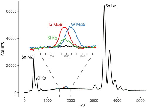
Figure 8 also shows that a further peak overlap is exhibited from the W Mαβ lines (Deslattes et al., 2003). In concentrations found in this study, these W peaks overlap significantly with the Si Kα peak such that misidentification of W for Si is also possible. In addition, the Sn Lα peaks (Lα₁ = 3.444 keV, Lα₂ = 3.436 keV; Deslattes et al., 2003) may produce a silicon escape peak of ∼1.7 keV, very nearly identical to the Si Kα peaks (Newbury, 2009).

For these reasons, and the lack of evidence found in this study, we conclude that the high Si contents reported by Hall and Ribbe (1971) and Moore and Howie (1979) are misidentified peaks, and that Si is a trace element at most (<50 ppm). We thus recommend its use in an inclusion detection suite during EPMA quality control routines for cassiterite analyses.

Equation 4: As pyrolusite (MnO₂) is another member of the rutile structure group, Mn⁴⁺ may be expected to exist favourably in the cassiterite lattice. This substitution is generally dismissed as requiring too high an f_O2 to occur in natural systems, in line with our modelled speciation curves for Mn (Figure 5c). No Mn was found outside of Nb–Ta coupled substitution mechanisms, nor has it been previously presented. Despite the theoretical plausibility from a lattice strain perspective (Figure 6a), this reaction does not need to be discussed further.

Equation 5: Incorporation of Ti⁴⁺ is undisputed and widely reported (Table 6), aided by the fact the both cassiterite and rutile (TiO₂) have the same crystal structure (Table 7). This is one of the dominant incorporation mechanisms for minor elements in cassiterite observed in this study, with the highest observed Ti contents of around 4 apfu*100 (Beechworth; Figure 2b). This is similar to the highest Ti contents previously reported by Hall and Ribbe (1971) of ∼3.5 apfu*100 (Table 1). The cassiterite–rutile solid solution series has been experimentally determined in the ceramics and materials science literature, with a solvus gap measured at 7 ± 4 mol% TiO₂ at 500 °C (Naidu & Virkar, 1998). The high Ti concentrations observed in some samples (e.g. Beechworth, Elsmore) appear to approach this upper limit of Ti solubility in natural cassiterite, however the mean concentrations within each sample are much lower (rarely exceeding 1 apfu*100). It is therefore likely that the dominant control on Ti concentration is a function of availability and partitioning during crystal growth, and not the upper solubility limit.

Equation 6: The existence of W⁴⁺ in cassiterite has been postulated previously (Table 6), however evidence to date has been either inconclusive (Hall & Ribbe, 1971; Möller et al., 1988) or not supportive (Černý et al., 2004). Synthetic samples of WO₂ show that the phase is monoclinic and thus not a member of the rutile structure group (Table 7), but it is a closely related structure with pairs of deformed WO₆ octahedra drawn together into doublets (Magnéli et al., 1955). This implies that the incorporation of W⁴⁺ into cassiterite might be favourable, in agreement with the lattice strain model (Figure 6).

Naturally occurring WO₂ is yet to be described (Pasero, 2020), and previous authors have generally assumed that W⁴⁺ requires too low of an f_O2 for natural Sn-bearing systems. However, the results of the thermodynamic modelling show that the transition from W⁴⁺ to W⁶⁺ as the dominant ionic species overlaps within the expected range of cassiterite mineralising systems (Figure 5b).

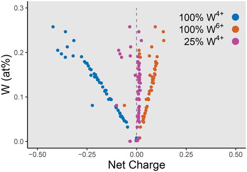
Stoichiometric evidence for the existence of W⁴⁺ is observed in Figure 7. An Fe- and Mn-free substitution mechanism is required for analyses that follow the y-axis, as is observed in the Saltwater Creek sample (Figure 7b). Calcium was included in the EPMA analytical routine for inclusion detection, and was not detected in these samples, ruling out micro inclusions of scheelite (CaWO₄) or a substitution mechanism of scheelite stoichiometry. It is possible that W in this case is substituting as W⁶⁺ with charge balance provided via a coupled substitution with Mg, or some other divalent cation not measured in this study. However, there is a clear correlation between W and the calculated deviation from charge neutrality, with a trend towards excess positive charge if all W is assumed to be hexavalent (Figure 9). Missing divalent cations are expected to plot in a trend towards excess negative charge. Another possibility is if two W⁶⁺ cations are accompanied by a nearby cationic vacancy (i.e. W⁶⁺W⁶⁺□ ⇌ 3Sn⁴⁺), and this reaction should plot vertically with zero net charge as a function of W content. Since neither of these trends are observed, charge cannot be balanced by the incorporation of other divalent or trivalent cations, such as Mg²⁺, and excess W uptake cannot be explained by a coupled vacancy substitution. Charge is instead only balanced for the Saltwater Creek sample if around 25% of the total W is tetravalent.

Figure 9. Net charge versus W for a cassiterite crystal from Saltwater Creek. The net charge is calculated as the sum of each component (in atomic percent) multiplied by their assumed charges (Nb⁵⁺, Ta⁵⁺, Sn⁴⁺, Ti⁴⁺, Zr⁴⁺, Fe²⁺, Mn²⁺), and assuming a stoichiometric concentration of 66.6̅ at% O. A linear correlation between charge and W concentration is observed. Charge is overbalanced (excess positive charge) if all W were assumed to be W⁶⁺, and underbalanced (excess negative charge) if all W were assumed to be W⁴⁺. Charge is only balanced if 25% of total W is W⁴⁺.

Although the incorporation of W⁴⁺ has generally been considered unlikely to occur (Möller et al., 1988), these three independent lines of evidence (stoichiometric observations, speciation calculations, and partition modelling) provide a compelling argument for the importance of homovalent W in cassiterite. Rather, the very high relative partition coefficient from our lattice strain model (D’ = 0.91; Figure 6) implies that, at least in Sn–W mineralising systems, higher concentrations of W should be detected than those observed for similar homovalent cations such as Ti, considering the D’ for Ti⁴⁺ is lower than W⁴⁺ (Figure 6) and that the W concentration of Sn–W mineralising fluids could be reasonably expected to be higher than the Ti concentration. This discrepancy may be due to the strong relationship between sector zonation and W distribution within cassiterite (Bennett et al., 2020), the effects of which are not considered within the lattice strain model. To our knowledge, this is the first reported evidence for W⁴⁺ in cassiterite. Further research into this mechanism should aim to confirm the oxidation state of W in these samples.

Equations 7 and 8: Homovalent substitution of Nb or Ta has previously been considered as a possible substitution mechanism in cassiterite, but analytical evidence was lacking (Möller et al., 1988). Synthetic Nb⁴⁺O₂ and Ta⁴⁺O₂ crystallise in the rutile structure group (Table 7; Rogers et al., 1969; Schönberg et al., 1954), although in this case the f_O2 required is interpreted to be too low for natural systems as these phases have not been found on Earth (as reported in the IMA CNMNC November 2020 list of approved minerals; Pasero, 2020).

The modelled speciation curves for Nb and Ta (Figure 5b) suggests that Ta⁴⁺ is extremely unlikely to occur in cassiterite mineral systems, requiring f_O2 conditions far below the QIF buffer. In contrast, the Nb speciation curve (Figure 5b) shows that while Nb⁵⁺ is the dominant species in these systems, a minor proportion of Nb⁴⁺ persists at low f_O2 conditions within the expected bounds of cassiterite mineral systems. In addition, the lattice strain model predicts a very high partition coefficient for Nb⁴⁺ (D’ = 0.989; Figure 6a).

In a binary plot between the sum of Fe and Mn versus the sum of Nb and Ta (Figure 10), the data are expected to lie along linear trends defined by the substitution mechanisms outlined in Table 5. Most samples lie along a 2:1 trend line due to a coupled substitution with divalent Fe or Mn (Equations 14–17, discussed below). However, a few samples (cassiterite from Moolyella, Bamboo Creek, and Emmons pegmatites; Figure 10a) plot above the 2:1 trend line. The existence of analyses above this line implies a necessary component of Nb or Ta-rich substitution, which is best explained via a component of Nb⁴⁺ or Ta⁴⁺ substitution. This ‘excess’ of Nb or Ta is also apparent in the Aberfoyle sample, which plots nearly parallel to the 2:1 trend line but is offset towards higher Nb + Ta values (Figure 10c).

Figure 10. Binary plots of the substitutional relationships between Fe + Mn and Nb + Ta. The grey trend lines represent slopes of 1:1 for the stoichiometric substitutions of Equations 10–13 and 2:1 for Equations 14–17. Substitution via Equations 1 and 2 will plot along the x-axis, likewise, substitution via Equations 7 and 8 will plot along the y-axis. Points plotting in regions defined between these lines require a component of each bounding substitutional stoichiometry. Samples are grouped according to (a) pegmatitic and granite-hosted systems, (b) greisen systems, (c) vein-hosted systems, and (d) skarn systems.

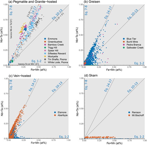
The modelled possibility of some Nb⁴⁺ being present during cassiterite mineralisation, and in consideration with the observed dominance of Nb over Ta in the Aberfoyle sample (Figure 3b, d), implies that Nb⁴⁺ is indeed a possible substitution mechanism in operation in natural cassiterite samples.

Equation 9: Zirconium is rarely reported in cassiterite EPMA data (Table 1), yet the direct homovalent substitution of Zr⁴⁺ into cassiterite is well known in the ceramics literature, with the solid solution series between SnO₂ and ZrO₂ reported to extend up to 25 at% ZrO₂ at 1100 °C (Dhage et al., 2006). While this temperature is much higher than the expected conditions of cassiterite mineral systems, the degree of solid solution is well beyond the maximum ∼0.08 at% found in the pegmatitic samples of this study. In the pegmatitic cassiterite crystals, which display the highest overall Zr concentration, the low intracrystalline variability (the population distribution of most samples are within analytical uncertainty of the mean; Figure 2c) suggests that Zr uptake is insensitive to environmental variables that result in the wide variability of other elements, and perhaps reflects less dynamic variables during crystallisation, such as temperature or pressure, or is buffered by the coexistence of zircon.

Pentavalent substitutions

This class has two subclasses of stoichiometry where this is possible. Firstly, an M⁵⁺X³⁺ coupled substitution may occur, displaying an M:X atomic ratio of 1:1 (Equations 10–13), which has no naturally occurring mineral analogue. Secondly, an M⁵⁺X²⁺ coupled substitution with a 2:1 atomic ratio (Equations 14–17), representing stoichiometry of the columbite group minerals (Table 7) is possible. The charge balancing cation (X) is usually reported as a combination of Fe and Mn, although any divalent or trivalent cation could fulfil this role.

Equations 10–13: In Figure 10, substitution mechanisms of this stoichiometry will plot along the 1:1 trend line. Most samples do not follow this trend, with only cassiterite from Trigg Hill and White Lode plotting on or near the 1:1 line (Figure 10a). Both of these have little to no Mn (Figure 3), thus Equations 10 and 11 (1:1 coupled (Nb,Ta)⁵⁺Fe³⁺) are the dominant substitutions mechanisms operating in these cassiterite samples. Indeed, the coupled substitution of pentavalent Nb and Ta with trivalent Mn (Equations 12 and 13) is very unlikely, due to the high f_O2 required (above FMQ; Figure 5c) for any significant amount of Mn³⁺ to occur.

Despite the dominance of the 2:1 trend line observed in cassiterite crystals from Poona Tin Shafts, Sifleetes Reward and Spear Hill (Figure 10a), the skew in slope towards the 1:1 trend line still requires a component of coupled (Nb,Ta)–Fe³⁺ substitutions (Equations 10 and 11). As such, while 1:1 (Nb,Ta)–Fe substitutions do not appear to be the dominant mechanism for the uptake of Nb, Ta and Fe into the cassiterite lattice, they are still important components to consider and should not be dismissed in favour of 2:1 (Nb,Ta)–Fe.

Equations 14–17: Most of the Nb–Ta contents in the cassiterite crystals of this study are coupled with Fe and Mn along a 2:1 trend line, including pegmatitic (Figure 10a), greisen (Figure 10b), and vein-hosted samples (Figure 10c). Such a strong uptake of (Nb,Ta)₂(Fe,Mn) is predicted by the lattice strain model (Figure 6b) with a D’ equal to unity, i.e. indistinguishable and fully interchangeable with Sn⁴⁺ itself.

The incorporation of Mn²⁺ via Equations 16 and 17 appears to be the dominant mechanism in which Mn is incorporated into the cassiterite lattice, due to the strong correlation with the 2:1 substitution trend line for the Mn-bearing pegmatitic samples (e.g. Spear Hill; Figure 10b).

The highest concentrations of Nb and Ta observed in cassiterite crystals of this study belong to pegmatitic mineral systems (Figures 3b, d and 10a), where cassiterite is well known to crystallise alongside columbite group minerals (CGM; Table 7). Previous authors have reported compositions of coexisting cassiterite–CGM pairs, as either inclusions of cassiterite in CGM or vice versa, and thus display the Mn and Ta contents of their cassiterite crystals within the columbite–tantalite quadrilateral (e.g. Masau et al., 2000; Neiva, 1996).

Only the pegmatitic cassiterite (Figure 11a), along with the crystals from the Blue Tier, Elsmore and Aberfoyle deposits (Figure 11b), contain sufficient Nb and Ta for comparison in this plot. The pegmatitic cassiterite crystals tend to cluster within a narrow range of Mn# and Ta#, and do not display evolutionary or fractionation trends as is commonly observed in the CGMs. An exception is Sifleetes Reward, which shows a wider range in Ta#, but comparable range in Mn# to the other pegmatitic samples. In contrast, the Blue Tier, Aberfoyle and Elsmore samples display considerable scatter.

Figure 11. Projection of cassiterite samples onto the columbite–tantalite quadrilateral, showing Mn# vs Ta#. The tapiolite–tantalite miscibility gap of Černý et al. (1992) is included for reference, with the dotted field representing the range of compositions between coexisting pairs of tantalite and tapiolite, and the grey dashed lines representing the compositional bounds for single phases. (a) Cassiterite from silicate liquid systems. (b) Cassiterite from hybrid and aqueous fluid systems.

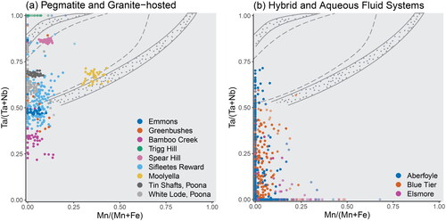
The tight clustering observed in the pegmatitic cassiterite samples may thus indicate a controlling presence of CGMs on the availability and uptake of Nb, Ta, Fe and Mn in those deposits, in particular the samples from Spear Hill and Moolyella, which plot along the miscibility gap of Černý et al. (1992).

Equations 18–19: It is also possible that W⁵⁺ may be incorporated into cassiterite via the 2:1 substitutional stoichiometry; however the pentavalent state for W is highly uncommon, reported mostly in the synthetic perovskite-structured ‘tungsten-bronzes’ (Okada et al., 2019 references therein). This exchange is not considered likely to play a significant role in geological systems, but the lattice strain model predicts a highly favourable relative partition coefficient (Figure 6b). A weak correlation is observed in Blue Tier and Saltwater Creek (Figure 7b) and Renison (Figure 7d) along a 2:1 trend line in the (Fe + Mn)–W binary plot. However, these trends are more likely to be spurious, due to coexisting substitutions with Nb and Ta.

The various coupled substitution mechanisms that exist between Fe, Mn, Nb and Ta can be stoichiometrically resolved using a W–(Fe,Mn)–(Nb,Ta) ternary plot (Figure 12), with the trend lines from the W–(Fe,Mn) binary projected along the W–(Fe,Mn) join. In Figure 12b, there is a partial trend in the Blue Tier sample, which appears to follow the hypothetical Eq18–Eq14 tie line, indicative of a component of W⁵⁺ (Equation 18). A similar, but weaker, trend is also seen in the Pedra Branca sample, but it is not observed in the Elsmore sample (Figure 12d) despite plotting in a similar region of the diagram. This correlation may instead reflect the total W⁶⁺/W⁴⁺ ratio, which coincidentally may be close to 0.5 for this sample (i.e. equal proportions of W⁶⁺ with W⁴⁺).

Figure 12. Ternary plots showing stoichiometric relationships between W, Fe + Mn, and Nb + Ta. These ternaries allow for comparison of W–Fe relationships in Nb + Ta bearing samples. The trend lines shown in Figure 10 project along the Fe + Mn and Nb + Ta join, and those shown in Figure 7 project along the Fe + Mn, and W join. Potential tie lines joining these substitutional stoichiometries are shown in grey. Transparency of the points decreases away from W concentrations at 2σ of the LLD, so that samples with the highest W contents are darker (more solid). Samples are grouped according to (a) pegmatitic and granite-hosted systems, (b) greisen systems, (c) vein-hosted systems, and (d) skarn systems.

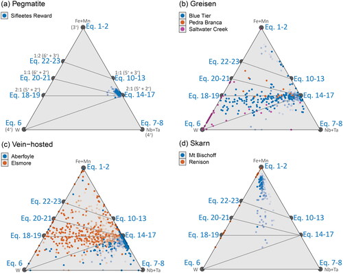
While these possible end member substitution reactions cannot be discriminated on the basis of stoichiometric considerations, a component of a reduced W species is still required to explain the W-rich behaviour observed. The Mn-poor nature of the W-rich samples in this study provides no evidence for or against Equation 19; nevertheless its role as a possible incorporation mechanism would be ruled out if further studies on these (or other) samples provide evidence against the incorporation of W⁵⁺.

Hexavalent substitutions

This class, exclusively for W⁶⁺ at the concentration levels considered in this work, also has two stoichiometric subclasses: an M⁶⁺X²⁺ coupled substitution for Sn with an M:X atomic ratio of 1:1 (Equations 20 and 21), and an M⁶⁺X³⁺X³⁺ coupled substitution with an M:X ratio of 1:2 (Equations 22 and 23). The charge balancing cation (X) is usually reported as a combination of Fe and Mn.

Equations 20 and 21: The main minerals of economic interest for W mineralisation are ferberite–hübnerite solid solution (wolframite) and scheelite (CaWO₄), in both of which W exists as W⁶⁺ (Table 7). Due to the prevalence of these minerals in Sn–W deposits, it would be expected that W in cassiterite follows a similar stoichiometric charge balance in a 1:1 coupled substitution mechanism with Fe or Ca. Since Ca was not detected in any of the cassiterite samples of this study, we will consider only the reactions involving Fe or Mn. Accordingly, the distribution of analyses should be restricted to the Fe-rich region above the Eq20–Eq14 tie line as seen in cassiterite from Sifleetes Reward (Figure 12a).

In general, this is not the case, and the samples most enriched in W plot below this line, indicative of a more W-rich substitution mechanism (as discussed above). This tie line does provide an upper bound to the Elsmore sample (Figure 12c) and may be the W⁶⁺ component for samples such as Blue Tier and Saltwater Creek if the existence of W⁵⁺ in Equation 18 were disproved in the future.

Equations 22 and 23: The 1:2 substitution mechanism has the stoichiometry of ‘oxiferberite’ (Fe³⁺₂WO₆) – a phase only known from anthropogenic origins and not yet found in nature (Chesnokov et al., 1998). None of the samples analysed in this study provide evidence for a coupled W⁶⁺–Fe³⁺ reaction (Equation 22). However, this may be due to a requirement of higher f_O2 conditions required than observed in this sample set, and so cannot be discounted.

The only sample in this study with enough W and Mn for discussion of the 1:1 (Equation 21) and 1:2 (Equation 23) coupled substitution mechanisms is the cassiterite crystal from Sifleetes Reward (Figure 12a). The strong clustering of samples above the Eq20–Eq14 tie line provides evidence for some component of Equation 21 (1:1 W:Mn²⁺); although this cannot be distinguished from Equation 20 (1:1 W:Fe²⁺) via stoichiometric analysis, the distinction between these substitution mechanisms is likely moot. As previously discussed, Mn³⁺ is unlikely to occur in cassiterite and thus this substitution mechanism (Equation 23, 1:2 W:Mn³⁺) is unlikely to occur in natural samples.

Paragenetic classification

In Figures 2 and 3, clear differences are observed between the minor element compositions of cassiterite crystals from different mineralising environments, such as a preference for Ti substitution in the cassiterite crystals associated with hydrothermal quartz vein systems. Figure 10 highlights how the Fe, Mn, Nb and Ta contents are most elevated in the pegmatitic cassiterite crystals, while some of the highest Fe contents are observed in the systems dominated by metasomatic processes (Mt Bischoff and Renison) in which the Fe³⁺ substitution reaction dominates. These differences may be exploited for a paragenetic classification diagram.

Extending the (Fe + Mn)–(Nb + Ta) binary system of Figure 10 into a ternary plot with Ti, substitutional ‘tie lines’ may be drawn between stoichiometric end-member points (Figure 13). For brevity and ease of reading, we have simplified the names of these tie lines to refer to only one possible substitution mechanism at each end, i.e. a tie line between Ti (Equation 5) and the 2:1 substitutional stoichiometries of Nb, Ta, Fe and Mn (Equations 14–17) is referred to as the Ti–Eq14 tie line.

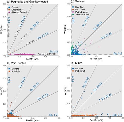
Figure 13. Ternary plots of the substitutional relationships between Ti, Fe + Mn, and Nb + Ta. The trend lines representing the 1:1 and 2:1 stoichiometric substitution reactions from Figure 10 project onto the Fe + Mn and Nb + Ta join, and tie lines joining these to the Ti apex are shown in grey. Colour represents the total SnO₂ content of each analysis, and the colour scheme was chosen to visually down-weight values close to stoichiometric SnO₂ (i.e. those with little to no substituting elements present). Samples are grouped according to (a) pegmatitic and granite-hosted systems, (b) greisen systems, (c) vein-hosted systems, and (d) skarn systems.

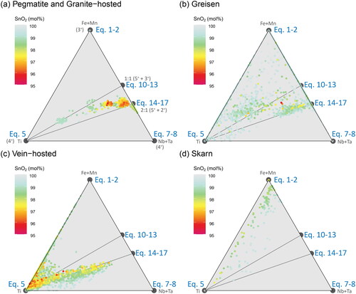
The pegmatite samples plot almost entirely within the region bound by the Ti–Eq10 and Ti–Eq14 tie lines (Figure 13a), although analyses from a few localities (specifically the Moolyella, Bamboo Creek and Emmons pegmatites) plot towards the Nb + Ta apex of the Eq14–(Nb,Ta) join. These are the same samples that plot above the 2:1 trend line in Figure 10a.

The greisen samples show two distinct populations (Figure 13b), one centred on the Ti–Eq14 tie line and the other on the Ti–Eq10 tie line, a relationship not apparent in the binary plot (Figure 10b). These clusters reflect transects through two different sector zones of the Blue Tier cassiterite crystal.

The vein-hosted samples show populations along the Ti–(Fe,Mn) join as well as along the Ti–Eq14 tie line, representing trivalent and divalent Fe substitution mechanisms, respectively (Figure 13c). The skarn samples plot nearest the Fe + Mn apex and display a diffuse trend towards Ti (Figure 13d), in corroboration of their overall high Fe concentrations, moderate Ti, and low Mn, Nb and Ta (Figures 2 and 3).

In Figure 14, probability density distribution contours for all analyses presented in this contribution are displayed as a function of the cassiterite mineral systems of our simplified physicochemical model. An overall pattern is observed: cassiterite crystals from Silicate Liquid Systems (pegmatites and granite-hosted disseminated Sn deposits; Figure 14a, b) plot dominantly near the Nb + Ta apex, and overlap with Hybrid systems (greisen deposits; Figure 14c) in a trend towards the Ti apex. These in turn overlap with the Aqueous Fluid Systems, where vein-hosted deposits cluster nearest to the Ti apex (Figure 14d), followed by skarn deposits along the join towards the Fe-apex (Figure 14e). This sequence likely reflects the decreasing availability of Nb and Ta as the mineralising environment evolves away from a silicate liquid dominated system towards an aqueous system dominated by magmatic fluids, followed by decreasing solubility of Ti and an increase in f_O2 due to mixing with meteoric fluids and/or significant wall-rock alteration towards skarn-style deposits.

Figure 14. The Ti–(Fe + Mn)–(Nb + Ta) ternary diagram from Figure 13, with the data from each sub-figure (Figure 13a–d) contoured as probability density distributions, coloured according to (a, b) pegmatite and granite-hosted disseminated Sn systems, (c) greisen systems, (d) vein systems, and (e) skarn systems. Analyses from the cassiterite crystal from Beechworth, which has an unknown paragenesis, are plotted as points with the same colour scheme as Figure 13.

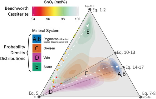
This figure may be used for classification of cassiterite crystals that are alluvial in nature, where the primary source is unidentified. For instance, the cassiterite from Beechworth was collected from Reedy Creek, which drains the biotite-granites of the Pilot Range to the north (Cochrane & Bowen, 1971; Dunn & Mahony, 1913). Numerous small dykes and veins of aplite, pegmatite, quartz and greisen are known within the Pilot Range granite, particularly to the northwest, associated with a quartz–tourmaline nodule granite (Birch, 1984; Cochrane & Bowen, 1971). However, none of these are large enough to be economic, and most with low grades that were prohibitive to small-scale mining operations of the early twentieth century (Dunn & Mahony, 1913). Cochrane and Bowen (1971) noted that cassiterite was found to be more common along Reedy Creek and the surrounding alluvial plains than was expected from these known mineralised bodies, and that the primary mineralised source for the cassiterite along the creek had not yet been identified. Cochrane and Bowen (1971) did not discount the possibility of a larger mineralised deposit, which may have been undiscovered or previously eroded, but generally favoured a model where the cassiterite is weathered from widespread low-grade dissemination within the granite.

Comparison of the Beechworth sample examined in this study with the results of Figure 14, shows that this crystal plots along the Ti–Fe join, with the highest concentrations of substituting elements (red points) plotting nearest to the Ti apex. This implies that the primary source of the Beechworth alluvial cassiterite is an aqueous-liquid dominated system, such as a vein or skarn deposit, and perhaps a greisen, but not a silicate-liquid dominated system such as a pegmatite, nor disseminated throughout the granite as magmatically precipitated cassiterite. If the source of cassiterite mineralisation at Beechworth were indeed from widespread, low-grade disseminations, and that this cassiterite crystal precipitated from aqueous fluids, then the mineralisation would possibly the result of pervasive alteration and breakdown of Sn-bearing biotite, resulting in localised deposition and precipitation of cassiterite. This hypothesis could be easily tested through petrographic examination of the parent granite in thin section, from samples widely spaced across the pluton. However, these results are from one crystal, and numerous crystals should be mapped and characterised (see the methods of Bennett et al., 2020) to ascertain the general population characteristics. Similarities between samples from different locations along the creek should also be considered, before a conclusive identification could be made.

Concluding remarks

On the basis of our observations and thermodynamic considerations, we discount 6 of the 23 possible substitution mechanisms initially described in Table 5 from occurring in natural cassiterite. These are the homovalent substitutions of Si⁴⁺ and Mn⁴⁺, and the coupled substitutions involving Mn³⁺. We find no supporting evidence for the charge balancing interstitial Fe and vacancy mechanism of Izoret et al. (1985) due to a lack of correlating Ti, and we cannot resolve the presence of W⁵⁺ via the stoichiometric methods employed here. Thus, we find that there are 14 possible substitution mechanisms for 7 minor elements into the cassiterite lattice. The variability of these numerous substitution mechanisms may be exploited as a record of the dynamic physicochemical processes that occurred during the growth of each cassiterite crystal. In particular, we discuss the variable speciation of Fe, W and Nb as a record of f_O2 below. These substitution mechanisms may also impart a unique fingerprint of the growth environment as a function of the specific cassiterite mineral system.

A record of oxygen fugacity

The existence of W- and Nb-rich samples, in excess of substituting Fe or Mn, suggests that the incorporation of these elements in the cassiterite lattice may be sensitive to the f_O2 of the system. This is dependent on the interpretation that the excess of these elements is due to their incorporation via their reduced M⁴⁺ states. If the oxidation state of these elements can be confirmed by other methods (e.g. TEM or XANES), then the W–(Fe,Mn)–(Nb,Ta) ternary diagram may be subdivided into regions of relative oxygen fugacity defined by the co-existence of Fe³⁺, Fe²⁺, W⁶⁺, W⁴⁺, (Nb,Ta)⁵⁺ and Nb⁴⁺.

The effect of sector zonation upon the preferential uptake of Fe²⁺ or Fe³⁺ via the two different Nb + Ta coupled substitution mechanisms means that the simple Fe²⁺/Fe³⁺ ratio cannot act as an effective indicator of oxygen fugacity. The W⁴⁺/W⁶⁺ ratio may be more effective in this regard, as there appears to be no preferential incorporation of W via different substitution mechanisms into different sectors of cassiterite crystals. In other words, W appears to partition strongly into the same sector regardless of oxidation state. Further work would be required to confirm the apparent W⁴⁺/W⁶⁺ ratio and if the calculation from stoichiometry (as in Figure 9, for example) is an accurate reflection of the true ratio, including measurement of the partition coefficients for each substitution mechanism. The magnitude of excess Nb may also be compared with the W⁴⁺/W⁶⁺ ratio, if the relative partition coefficients for Nb⁴⁺ and the coupled Nb⁵⁺ substitution mechanisms are also measured experimentally in future studies.

While not identified in any sample of this study, the presence of any Mn³⁺ (or even Mn⁴⁺) in cassiterite would be strong evidence for higher f_O2 systems (>NNO). This is not expected for most granite-related Sn systems, and instead might be an indicator of processes such as cassiterite precipitation driven by oxidation of Sn-bearing sulfide ores. As such, if Mn³⁺ were to be detected in cassiterite grains targeted for isotopic dating, for example, then the veracity of those ages would be questionable. This hypothesis could be tested in future studies on cassiterite, targeting cassiterite crystals from a range of crystallisation methods not examined within this study.

Fingerprinting cassiterite mineral systems

The preliminary results of this contribution suggest that the Ti–(Fe,Mn)–(Nb,Ta) ternary plot may be a useful discrimination or classification diagram, which may be used to constrain alluvially collected cassiterite to one of the cassiterite mineral systems of our simplified model. Such knowledge may prove valuable for target generation and tenement acquisition for cassiterite bearing mineral deposits, and to aid decision making during exploration and drilling campaigns. For example, if the primary source of the Beechworth alluvial Sn deposit were suspected to be an economically exploitable deposit, rather than low-grade disseminations, and was the subject of an exploration campaign, then initial targeting of sites proximal to the granite-host rock contact (preferably near shale or carbonate sequences) may prove to be the fastest discovery route, rather than targeting known pegmatite swarms.

Future research

Future analyses of cassiterite should include transects across growth zones, taking into account growth zone variability as noted in Bennett et al. (2020) to further constrain the validity and limitations of the Ti–(Fe,Mn)–(Nb,Ta) ternary classification diagram. Detailed studies on the chemistry of multiple cassiterite crystals throughout differing paragenetic sequences, modes of emplacement and position within the system for a single locality (rather than studies on cassiterite crystals from across numerous localities, such as this one) will highlight deposit scale variability and allow for comparison with regional systematic trends. The W–(Fe,Mn)–(Nb,Ta) ternary redox diagram could be tested through direct measurement of the oxidation states of Fe, Mn, W, Nb and Ta via either Transition Electron Microscope (TEM) Electron Energy Loss Spectroscopy (EELS) or synchrotron XANES methods. Another approach via experimentally grown cassiterite crystals is also possible. Combined with cassiterite U–Pb (Liu et al., 2007; Moscati & Neymark, 2020; Neymark et al., 2018), δ¹⁸O (Carr et al., 2017), and Hf-isotope systematics (Kendall-Langley et al., 2020), minor element systematics are another promising addition to the cassiterite ‘multitool’.

Code and data availability

All data files and analytical code referred to in this manuscript is available in the GitHub repository: github.com/orthospar/MinorElements-Cassiterite. The clean (final) EPMA data file is also available online as a supplementary file.

Sample availability

All samples have been registered with the Edward de Courcy Clarke Earth Science Museum at the University of Western Australia. Registration details are available in a supplementary file in the GitHub repository github.com/orthospar/MinorElements-Cassiterite.

Author contributions

JMB and AISK conceived the study, with the research executed and manuscript prepared by JMB in a doctoral study under the guidance of AISK, SGH, and MLF. AISK, SGH, MLF and MPR provided input and comments on draft versions of this manuscript. MPR also provided direction and guidance with the operation of the Electron Probe and subsequent data reduction methodologies.

Acknowledgements

The authors would like to thank Lisard Torró, Simon Goldmann, Antony Burnham, and an anonymous reviewer, for their helpful comments on this manuscript, which also benefited from valuable discussions with Jon Blundy, Andrew G. Christy, Robert Loucks and Franco Pirajno. The authors also thank Geert Beuters, Nilson F. Bothelo, Stewart Cole, Sue Koepke, Matthew Latham and Nigel Richardson for provision of some samples used in this study. The authors acknowledge the facilities and the scientific and technical assistance of the Australian Microscopy & Microanalysis Research Facility at the Centre for Microscopy, Characterisation & Analysis, The University of Western Australia, a facility funded by the University, State and Commonwealth Governments.

Disclosure statement

The authors report there are no competing interests to declare.

Additional information

Funding

Jason M. Bennett was supported by an Australian Government Research Training Program (RTP) Scholarship. Jason M. Bennett and Marco L. Fiorentini also acknowledge support from the Australian Research Council through the ARC Centre of Excellence for Core to Crust Fluid Systems (CE110001017).

References

- Africano, F., Rompaey, G. V., Bernard, A., & Guern, F. L. (2014). Deposition of trace elements from high temperature gases of Satsuma-Iwojima volcano. Earth, Planets and Space, 54(3), 275–286. https://doi.org/10.1186/BF03353027
- Ahmad, M. (1995). Genesis of tin and tantalum mineralization in pegmatites from the Bynoe area, Pine Creek Geosyncline, Northern Territory. Australian Journal of Earth Sciences, 42(5), 519–534. https://doi.org/10.1080/08120099508728222
- Allison, T. C. (2013). NIST-JANAF Thermochemical Tables – SRD 13 (1.0.2) [dataset]. National Institute of Standards and Technology. https://doi.org/10.18434/T42S31
- Benites, D., Torró, L., Vallance, J., Laurent, O., Quispe, P., Rosas, S., Uzieda, M. F., Holm-Denoma, C. S., Pianowski, L. S., Camprubí, A., Colás, V., Fernández-Baca, A., Giraldo, L., Chelle-Michou, C., Sáez, J., Kouzmanov, K., & Fontboté, L. (2022). Geology, mineralogy, and cassiterite geochronology of the Ayawilca Zn–Pb–Ag–In–Sn–Cu deposit, Pasco, Peru. Mineralium Deposita, 57(3), 481–507. https://doi.org/10.1007/s00126-021-01066-z
- Bennett, J. M., Kemp, A. I. S., & Roberts, M. P. (2020). Microstructural controls on the chemical heterogeneity of cassiterite revealed by cathodoluminescence and elemental X-ray mapping. American Mineralogist, 105(1), 58–76. https://doi.org/10.2138/am-2020-6964
- Bhalla, P., Holtz, F., Linnen, R. L., & Behrens, H. (2005). Solubility of cassiterite in evolved granitic melts: Effect of t, fO2, and additional volatiles. Lithos, 80(1-4), 387–400. https://doi.org/10.1016/j.lithos.2004.06.014
- Birch, W. D. (1984). Quartz–topaz–loellingite rocks near Eldorado, Victoria. Australian Journal of Earth Sciences, 31(3), 269–278. https://doi.org/10.1080/14400958408527929
- Blevin, P. L., & Norman, M. D. (2010). Cassiterite: The zircon of mineral systems – A scoping study. Poster.
- Blissett, A. H. (1959). The geology of the Rossarden-Storeys Creek District (Geological Survey of Tasmania, Bulletin No. 46). Tasmanian Department of Mines.
- Blundy, J. D., & Wood, B. J. (1994). Prediction of crystal-melt partition coefficients from elastic moduli. Nature, 372(6505), 452–454. https://doi.org/10.1038/372452a0
- Blundy, J. D., & Wood, B. J. (2003). Partitioning of trace elements between crystals and melts. Earth and Planetary Science Letters, 210(3-4), 383–397. https://doi.org/10.1016/s0012-821x(03)00129-8
- Bolzan, A. A., Fong, C., Kennedy, B. J., & Howard, C. J. (1997). Structural studies of rutile-type metal dioxides. Acta Crystallographica Section B Structural Science, 53(3), 373–380. https://doi.org/10.1107/S0108768197001468
- Botelho, N. F., & Moura, M. A. (1998). Granite-ore deposit relationships in Central Brazil. Journal of South American Earth Sciences, 11(5), 427–438. https://doi.org/10.1016/s0895-9811(98)00026-1
- Breiter, K., Korbelová, Z., Chládek, Š., Uher, P., Knesl, I., Rambousek, P., Honig, S., & Šešulka, V. (2017). Diversity of Ti–Sn–W–Nb–Ta oxide minerals in the classic granite-related magmatic–hydrothermal Cínovec/Zinnwald Sn–W–Li deposit (Czech Republic). European Journal of Mineralogy, 29(4), 727–738. https://doi.org/10.1127/ejm/2017/0029-2650
- Brown, R. E., Stroud, W. J. (1993). Mineralisation related to the Gilgai Granite, Tingha-Inverell area. New England Orogen 1993 Conference Proceedings, 431–447.
- Carr, P. A., Norman, M. D., & Bennett, V. C. (2017). Assessment of crystallographic orientation effects on secondary ion mass spectrometry (SIMS) analysis of cassiterite. Chemical Geology, 467, 122–133. https://doi.org/10.1016/j.chemgeo.2017.08.003
- Černý, P., Blevin, P. L., Cuney, M., & London, D. (2005). Granite-related ore deposits. In J. W. Hedenquist, J. F. H. Thompson, R. J. Goldfarb & J. P. Richards (Eds.), Economic Geology, 100th Anniversary Volume (pp. 337–370). Society of Economic Geologists.
- Černý, P., Chapman, R., Ferreira, K., & Smeds, S.-A. (2004). Geochemistry of oxide minerals of Nb, Ta, Sn, and Sb in the Varuträsk granitic pegmatite, Sweden: The case of an anomalous columbite–tantalite trend. American Mineralogist, 89(4), 505–518. https://doi.org/10.2138/am-2004-0405
- Černý, P., & Ercit, T. S. (2005). The classification of granitic pegmatites revisited. The Canadian Mineralogist, 43(6), 2005–2026. https://doi.org/10.2113/gscanmin.43.6.2005
- Černý, P., Ercit, T. S., & Wise, M. A. (1992). The tantalite–tapiolite gap; natural assemblages versus experimental data. The Canadian Mineralogist, 30(3), 587–596.
- Chakhmouradian, A. R., Smith, M. P., & Kynicky, J. (2015). From “strategic" tungsten to “green" neodymium: A century of critical metals at a glance. Ore Geology Reviews, 64, 455–458. https://doi.org/10.1016/j.oregeorev.2014.06.008
- Chang, E., & Graham, E. K. (1975). The elastic constants of cassiterite SnO2 and their pressure and temperature dependence. Journal of Geophysical Research, 80(17), 2595–2599. https://doi.org/10.1029/JB080i017p02595
- Chao, E. C. T., Fahey, J. J., Littler, J., & Milton, D. J. (1962). Stishovite, SiO2, a very high pressure new mineral from Meteor Crater, Arizona. Astrogeologic Studies: Annual Progress Report. Crater Investigations. Part B, 10.
- Chappell, B. W., & White, A. J. R. (2001). Two contrasting granite types: 25 years later. Australian Journal of Earth Sciences, 48(4), 489–499. https://doi.org/10.1046/j.1440-0952.2001.00882.x
- Cheng, Y., Mao, J., Chang, Z., & Pirajno, F. (2013). The origin of the world class tin–polymetallic deposits in the Gejiu district, SW China: Constraints from metal zoning characteristics and 40Ar–39Ar geochronology. Ore Geology Reviews, 53, 50–62. https://doi.org/10.1016/j.oregeorev.2012.12.008
- Cheng, Y., Spandler, C., Kemp, A., Mao, J., Rusk, B., Hu, Y., & Blake, K. (2019). Controls on cassiterite (SnO2) crystallization: Evidence from cathodoluminescence, trace-element chemistry, and geochronology at the Gejiu Tin District. American Mineralogist, 104(1), 118–129. https://doi.org/10.2138/am-2019-6466
- Chesnokov, B., Kotrly, M., & Nisanbajev, T. (1998). Brennende abraumhalden und aufschlüsse im Tscheljabinsker kohlenbecken – eine reiche mineralienküche. Mineralien-Welt, 9(3), 54–63.
- Cochrane, G. W., & Bowen, K. G. (1971). Tin deposits of Victoria (pp. 1–72). Geological Survey of Victoria, Bulletin No. 60. Victorian Department of Mines.
- Darwin, C. R. (1857). Letter no. 2130. https://www.darwinproject.ac.uk/letter/DCP-LETT-2130.xml
- Deslattes, R. D., Kessler, E. G., Indelicato, P., Billy, L. d., Lindroth, E., & Anton, J. (2003). X-ray transition energies: New approach to a comprehensive evaluation. Reviews of Modern Physics, 75(1), 35–99. https://doi.org/10.1103/RevModPhys.75.35
- Dhage, S. R., Samuel, V., Pasricha, R., & Ravi, V. (2006). Studies on SnO2–ZrO2 solid solution. Ceramics International, 32(8), 939–941. https://doi.org/10.1016/j.ceramint.2005.06.012
- Dohmen, R., Faak, K., & Blundy, J. D. (2017). Chronometry and speedometry of magmatic processes using chemical diffusion in olivine, plagioclase and pyroxenes. Reviews in Mineralogy and Geochemistry, 83(1), 535–575. https://doi.org/10.2138/rmg.2017.83.16
- Donovan, J. J. (2018). CalcImage (Version 12.3.7). Probe Software, Inc.
- Duc-Tin, Q., Audétat, A., & Keppler, H. (2007). Solubility of tin in (Cl, F)-bearing aqueous fluids at 700 °C, 140 MPa: A LA-ICP-MS study on synthetic fluid inclusions. Geochimica et Cosmochimica Acta, 71(13), 3323–3335. https://doi.org/10.1016/j.gca.2007.04.022
- Dunn, E. J., & Mahony, D. J. (1913). The Woolshed Valley, Beechworth (pp. 1–72). Geological Survey of Victoria, Bulletin No. 25. Victorian Department of Mines.
- Dusausoy, Y., Ruck, R., & Gaite, J. M. (1988). Study of the symmetry of Fe3+ sites in SnO2 by electron paramagnetic resonance. Physics and Chemistry of Minerals, 15(3), 300–303. https://doi.org/10.1007/BF00307520
- Ercit, T. S., Wise, M. A., & Cerny, P. (1995). Compositional and structural systematics of the columbite group. American Mineralogist, 80(5-6), 613–619. https://doi.org/10.2138/am-1995-5-619
- Falster, A. U., Simmons, W. B., Webber, K. L., Dallaire, D. A., Nizamoff, J. W., & Sprague, R. A. (2019). The Emmons pegmatite, Greenwood, Oxford County, Maine. Rocks & Minerals, 94(6), 498–519. https://doi.org/10.1080/00357529.2019.1641021
- Farmer, C. B., Searl, A., & Halls, C. (1991). Cathodoluminescence and growth of cassiterite in the composite lodes at South Crofty Mine, Cornwall, England. Mineralogical Magazine, 55(380), 447–458. https://doi.org/10.1180/minmag.1991.055.380.14
- Galliski, M. A., Marquez-Zavalia, M. F., Cerny, P., Martinez, V. A., & Chapman, R. (2008). The Ta–Nb–Sn–Ti oxide-mineral paragenesis from La Viquita, a spodumene-bearing rare-element granitic pegmatite, San Luis, Argentina. The Canadian Mineralogist, 46(2), 379–393. https://doi.org/10.3749/canmin.46.2.379
- Groves, D. I., Cocker, J. D., & Jennings, D. (1977). The Blue Tier Batholith. Geological Survey of Tasmania, Bulletin No. 55. Tasmania Department of Mines.
- Grundmann, G., & Morteani, G. (1998). Alexandrite, emerald, ruby, sapphire and topaz in a biotite–phlogopite fels from Poona, Cue District, Western Australia. Australian Gemmologist, 20, 159–167.
- Guo, J., Zhang, R., Li, C., Sun, W., Hu, Y., Kang, D., & Wu, J. (2018). Genesis of the Gaosong Sn–Cu deposit, Gejiu district, SW China: Constraints from in situ LA-ICP-MS cassiterite U–Pb dating and trace element fingerprinting. Ore Geology Reviews, 92, 627–642. https://doi.org/10.1016/j.oregeorev.2017.11.033
- Guo, J., Zhang, R., Sun, W., Ling, M., Hu, Y., Wu, K., Luo, M., & Zhang, L. (2018). Genesis of tin-dominant polymetallic deposits in the Dachang district, South China: Insights from cassiterite U–Pb ages and trace element compositions. Ore Geology Reviews, 95, 863–879. https://doi.org/10.1016/j.oregeorev.2018.03.023
- Hagemann, S. G., Lisitsin, V. A., & Huston, D. L. (2016). Mineral system analysis: Quo vadis. Ore Geology Reviews, 76, 504–522. https://doi.org/10.1016/j.oregeorev.2015.12.012
- Hall, M. R. (1968). An electron microprobe study of luminescence centers in cassiterite [Master’s thesis]. Virginia Polytechnic Institute.
- Hall, M. R., & Ribbe, P. H. (1971). An electron microprobe study of luminescence centers in cassiterite. American Mineralogist, 56(1-2), 31–45.
- Halley, S. W., & Walshe, J. L. (1995). A reexamination of the Mount Bischoff cassiterite sulfide skarn, western Tasmania. Economic Geology, 90(6), 1676–1693. https://doi.org/10.2113/gsecongeo.90.6.1676
- Hamilton, N. (2017). Ggtern: An extension to ‘ggplot2’, for the creation of ternary diagrams. https://CRAN.R-project.org/package=ggtern
- Heinrich, C. A. (1990). The chemistry of hydrothermal tin(–tungsten) ore deposition. Economic Geology, 85(3), 457–481. https://doi.org/10.2113/gsecongeo.85.3.457
- Hennigh, Q., & Hutchinson, R. W. (1999). Cassiterite at Kidd Creek: An example of volcanogenic massive sulfide-hosted tin mineralization. In M. D. Hannington & C. T. Barrie (Eds.), The Giant Kidd Creek Volcanogenic Massive Sulfide Deposit, Western Abitibi Subprovince, Canada, Monograph Series 10. Society of Economic Geologists. https://doi.org/10.5382/Mono.10.17
- Hong, W., Cooke, D. R., Zhang, L., Fox, N., & Thompson, J. (2021). The formation of magmatic-hydrothermal features in Sn-mineralized and barren Tasmanian intrusions, southeast Australia: Insights from quartz textures, trace elements, and microthermometry. Economic Geology, 116(8), 1917–1948. https://doi.org/10.5382/econgeo.4853
- Hutchinson, R. W. (1982). Geologic setting and genesis of cassiterite-sulfide mineralization at Renison Bell, Western Tasmania. Economic Geology, 77(1), 199–202. https://doi.org/10.2113/gsecongeo.77.1.199
- Ishihara, S. (1979). Lateral variation of magnetic susceptibility of the Japanese granitoids. The Journal of the Geological Society of Japan, 85(8), 509–523. https://doi.org/10.5575/geosoc.85.509
- Izoret, L., Marnier, G., & Dusausoy, Y. (1985). Caracterisation cristallochimique de la cassiterite des gisements d’etain et de tungstene de Galice, Espagne. The Canadian Mineralogist, 23(2), 221–231.
- Jacobson, M. I., Calderwood, M. A., & Grguric, B. A. (2007). Guidebook to the pegmatites of Western Australia. Hesperian Press.
- Jambor, J. L., Pertsev, N. N., & Roberts, A. C. (1995). New mineral names. American Mineralogist, 80(7-8), 845–850.
- Keid, H. G. W. (1951). Memorandum—investigation lease no. 31M/50 Coles Bay [MRT document UR1951 070 73]. Mineral Resources Tasmania.
- Kelly, W. C., & Rye, R. O. (1979). Geologic, fluid inclusion, and stable isotope studies of the tin–tungsten deposits of Panasqueira, Portugal. Economic Geology, 74(8), 1721–1822. https://doi.org/10.2113/gsecongeo.74.8.1721
- Kendall-Langley, L. A., Kemp, A. I. S., Grigson, J. L., & Hammerli, J. (2020). U–Pb and reconnaissance Lu–Hf isotope analysis of cassiterite and columbite group minerals from Archean Li–Cs–Ta type pegmatites of Western Australia. Lithos, 352-353, 105231. https://doi.org/10.1016/j.lithos.2019.105231
- Lenharo, S. L. R., Moura, M. A., & Botelho, N. F. (2002). Petrogenetic and mineralization processes in Paleo- to Mesoproterozoic rapakivi granites: Examples from Pitinga and Goiás, Brazil. Precambrian Research, 119(1-4), 277–299. https://doi.org/10.1016/s0301-9268(02)00126-2
- Linnen, R. L., Pichavant, M., Holtz, F., & Burgess, S. (1995). The effect of fO2 on the solubility, diffusion, and speciation of tin in haplogranitic melt at 850 °C and 2 kbar. Geochimica et Cosmochimica Acta, 59(8), 1579–1588. https://doi.org/10.1016/0016-7037(95)00064-7
- Liu, Y. P., Li, Z. X., Li, H. M., Guo, L. G., Xu, W., Ye, L., Li, C. Y., & Pi, D. H. (2007). U–Pb geochronology of cassiterite and zircon from the Dulong Sn–Zn deposit: Evidence for Cretaceous large-scale granitic magmatism and mineralization events in southeastern Yunnan province, China. Acta Petrologica Sinica, 23, 967–976.
- London, D. (2014). A petrologic assessment of internal zonation in granitic pegmatites. Lithos, 184-187, 74–104. https://doi.org/10.1016/j.lithos.2013.10.025
- Losos, Z., & Beran, A. (2004). OH defects in cassiterite. Mineralogy and Petrology, 81(3-4), 219–234. https://doi.org/10.1007/s00710-004-0040-x
- Lufkin, J. L. (1976). Oxide minerals in miarolitic rhyolite, Black Range, New Mexico. American Mineralogist, 61(5-6), 425–430.
- Lufkin, J. L. (1977). Chemistry and mineralogy of wood-tin, Black Range, New Mexico. American Mineralogist, 62(1-2), 100–106.
- Magnéli, A., Andersson, G., Blomberg, B., & Kihlborg, L. (1952). Identification of molybdenum and tungsten oxides by x-ray powder patterns. Analytical Chemistry, 24(12), 1998–2000. https://doi.org/10.1021/ac60072a039
- Magnéli, A., Andersson, G., Sundkvist, G., & Sundkvist, G. (1955). On the MoO2 structure type. Acta Chemica Scandinavica, 9(1), 1378–1381. https://doi.org/10.3891/acta.chem.scand.09-1378
- Maldener, J., Rauch, F., Gavranic, M., & Beran, A. (2001). OH absorption coefficients of rutile and cassiterite deduced from nuclear reaction analysis and FTIR spectroscopy. Mineralogy and Petrology, 71(1-2), 21–29. https://doi.org/10.1007/s007100170043
- Marshall, D., Downes, P., Ellis, S., Greene, R., Loughrey, L., & Jones, P. (2016). Pressure-temperature-fluid constraints for the Poona Emerald Deposits, Western Australia: Fluid inclusion and stable isotope studies. Minerals, 6(4), 130. https://doi.org/10.3390/min6040130
- Masau, M., Cerny, P., & Chapman, R. (2000). Exsolution of zirconian–hafnian wodginite from manganoan–tantalian cassiterite, Annie Claim #3 Granitic Pegmatite, Southeastern Manitoba, Canada. The Canadian Mineralogist, 38(3), 685–694. https://doi.org/10.2113/gscanmin.38.3.685
- Matjuschkin, V., Blundy, J. D., & Brooker, R. A. (2016). The effect of pressure on sulphur speciation in mid- to deep-crustal arc magmas and implications for the formation of porphyry copper deposits. Contributions to Mineralogy and Petrology, 171(7), Article 66. https://doi.org/10.1007/s00410-016-1274-4
- Meinert, L. D., Dipple, G. M., & Nicolescu, S. (2005). World skarn deposits. In J. W. Hedenquist, J. F. H. Thompson, R. J. Goldfarb & J. P. Richards (Eds.), Economic Geology, 100th Anniversary Volume (pp. 299–366). Society of Economic Geologists.
- Mercer, C. N., Reed, M. H., & Mercer, C. M. (2015). Time scales of porphyry Cu deposit formation: Insights from titanium diffusion in quartz. Economic Geology, 110(3), 587–602. https://doi.org/10.2113/econgeo.110.3.587
- Möller, P., Dulski, P., Szacki, W., Malow, G., & Riedel, E. (1988). Substitution of tin in cassiterite by tantalum, niobium, tungsten, iron and manganese. Geochimica et Cosmochimica Acta, 52(6), 1497–1503. https://doi.org/10.1016/0016-7037(88)90220-7
- Moore, F., & Howie, R. A. (1979). Geochemistry of some Cornubian cassiterites. Mineralium Deposita, 14(1), 103–107. https://doi.org/10.1007/BF00201869
- Moscati, R. J., & Neymark, L. A. (2020). U–Pb geochronology of tin deposits associated with the Cornubian Batholith of southwest England: Direct dating of cassiterite by in situ LA-ICPMS. Mineralium Deposita, 55(1), 1–20. https://doi.org/10.1007/s00126-019-00870-y
- Naidu, H. P., & Virkar, A. V. (1998). Low-temperature TiO2–SnO2 phase diagram using the molten-salt method. Journal of the American Ceramic Society, 81(8), 2176–2180. https://doi.org/10.1111/j.1151-2916.1998.tb02603.x
- Nambaje, C., Eggins, S. M., Yaxley, G. M., & Sajeev, K. (2020). Micro-characterisation of cassiterite by geology, texture and zonation: A case study of the Karagwe Ankole belt, Rwanda. Ore Geology Reviews, 124, 103609. https://doi.org/10.1016/j.oregeorev.2020.103609
- Neiva, A. M. R. (1996). Geochemistry of cassiterite and its inclusions and exsolution products from tin and tungsten deposits in Portugal. The Canadian Mineralogist, 34(4), 745–768.
- Neiva, A. M. R. (2008). Geochemistry of cassiterite and wolframite from tin and tungsten quartz veins in Portugal. Ore Geology Reviews, 33(3-4), 221–238. https://doi.org/10.1016/j.oregeorev.2006.05.013
- Newbury, D. E. (2009). Mistakes encountered during automatic peak identification of minor and trace constituents in electron-excited energy dispersive X-ray microanalysis. Scanning, 31(3), 91–101. https://doi.org/10.1002/sca.20151
- Neymark, L. A., Holm-Denoma, C. S., & Moscati, R. J. (2018). In situ LA-ICPMS U–Pb dating of cassiterite without a known-age matrix-matched reference material: Examples from worldwide tin deposits spanning the Proterozoic to the Tertiary. Chemical Geology, 483, 410–425. https://doi.org/10.1016/j.chemgeo.2018.03.008
- Okada, M., Ono, K., Yoshio, S., Fukuyama, H., & Adachi, K. (2019). Oxygen vacancies and pseudo Jahn-Teller destabilization in cesium-doped hexagonal tungsten bronzes. Journal of the American Ceramic Society, 102(9), 5386–5400. https://doi.org/10.1111/jace.16414
- Pal, D. C., Mishra, B., & Bernhardt, H.-J. (2007). Mineralogy and geochemistry of pegmatite-hosted Sn-, Ta–Nb-, and Zr–Hf-bearing minerals from the southeastern part of the Bastar-Malkangiri pegmatite belt, Central India. Ore Geology Reviews, 30(1), 30–55. https://doi.org/10.1016/j.oregeorev.2005.10.004
- Partington, G. A., McNaughton, N. J., & Williams, I. S. (1995). A review of the geology, mineralization, and geochronology of the Greenbushes Pegmatite, Western Australia. Economic Geology, 90(3), 616–635. https://doi.org/10.2113/gsecongeo.90.3.616
- Pasero, M. (2020). The new IMA list of minerals, November 2020. IMA CNMNC. http://cnmnc.main.jp/
- Pavlova, G. G., Palessky, S. V., Borisenko, A. S., Vladimirov, A. G., Seifert, T., & Phan, L. A. (2015). Indium in cassiterite and ores of tin deposits. Ore Geology Reviews, 66, 99–113. https://doi.org/10.1016/j.oregeorev.2014.10.009
- Pekov, I. V., Koshlyakova, N. N., Zubkova, N. V., Lykova, I. S., Britvin, S. N., Yapaskurt, V. O., Agakhanov, A. A., Shchipalkina, N. V., Turchkova, A. G., & Sidorov, E. G. (2018). Fumarolic arsenates – a special type of arsenic mineralization. European Journal of Mineralogy, 30(2), 305–322. https://doi.org/10.1127/ejm/2018/0030-2718
- Piranjo, F. (2009). Hydrothermal processes and mineral systems. Springer.
- Reid, A. M., & Henderson, Q. J. (1928). Blue Tier Tin Field. Geological Survey of Tasmania, Bulletin No. 38. Tasmania Department of Mines. Hobart.
- Ritchie, N. W. M. (2009). Spectrum simulation in DTSA-II. Microscopy and Microanalysis, 15(5), 454–468. https://doi.org/10.1017/s1431927609990407
- Ritchie, N. W. M. (2019). DTSA-II (Lorentz). NIST. https://www.cstl.nist.gov/div837/837.02/epq/dtsa2/index.html
- Rogers, D. B., Shannon, R. D., Sleight, A. W., & Gillson, J. L. (1969). Crystal chemistry of metal dioxides with rutile-related structures. Inorganic Chemistry, 8(4), 841–849. https://doi.org/10.1021/ic50074a029
- Ruck, R., Dusausoy, Y., Trung, C. N., Gaite, J.-M., & Murciego, A. (1989). Powder EPR study of natural cassiterites and synthetic SnO2 doped with Fe, Ti, Na and Nb. European Journal of Mineralogy, 1(3), 343–352. https://doi.org/10.1127/ejm/1/3/0343
- Schmidt, C. (2018). Formation of hydrothermal tin deposits: Raman spectroscopic evidence for an important role of aqueous Sn(IV) species. Geochimica et Cosmochimica Acta, 220, 499–511. https://doi.org/10.1016/j.gca.2017.10.011
- Schönberg, N., Overend, W. G., Munthe-Kaas, A., & Sörensen, N. A. (1954). An X-ray investigation of the tantalum-oxygen system. Acta Chemica Scandinavica, 8, 240–245. https://doi.org/10.3891/acta.chem.scand.08-0240
- Serranti, S., Ferrini, V., Masi, U., & Cabri, L. J. (2002). Trace-element distribution in cassiterite and sulfides from Rubane and massive ores of the Corvo deposit, Portugal. The Canadian Mineralogist, 40(3), 815–835. https://doi.org/10.2113/gscanmin.40.3.815
- Shannon, R. D. (1976). Revised effective ionic radii and systematic studies of interatomic distances in halides and chalcogenides. Acta Crystallographica Section A, 32(5), 751–767. https://doi.org/10.1107/S0567739476001551
- Shannon, R. D., & Prewitt, C. T. (1969). Effective ionic radii in oxides and fluorides. Acta Crystallographica Section B Structural Crystallography and Crystal Chemistry, 25(5), 925–946. https://doi.org/10.1107/S0567740869003220
- Sharko, E. D. (1971). Nature and properties of varlamoffite (oxidation products of stannite). International Geology Review, 13(4), 603–614. https://doi.org/10.1080/00206817109475474
- Summers, K. W. A. (1957). The mineral deposits of West Arm, Bynoe Harbour and Bamboo Creek Field, Northern Territory (BMR Record 1957/68). Bureau of Mineral Resources Geology and Geophysics.
- Sweetapple, M. T., & Collins, P. L. F. (2002). Genetic framework for the classification and distribution of Archean rare metal pegmatites in the North Pilbara Craton, Western Australia. Economic Geology, 97(4), 873–895. https://doi.org/10.2113/gsecongeo.97.4.873
- Swope, R. J., Smyth, J. R., & Larson, A. C. (1995). H in rutile-type compounds: I. Single-crystal neutron and X-ray diffraction study of H in rutile. American Mineralogist, 80(5-6), 448–453. https://doi.org/10.2138/am-1995-5-604
- Taylor, R. G. (1979). Geology of tin deposits. Elsevier Science.
- Thomas, J. B., Bruce Watson, E., Spear, F. S., Shemella, P. T., Nayak, S. K., & Lanzirotti, A. (2010). TitaniQ under pressure: The effect of pressure and temperature on the solubility of Ti in quartz. Contributions to Mineralogy and Petrology, 160(5), 743–759. https://doi.org/10.1007/s00410-010-0505-3
- Thomas, R., & Davidson, P. (2016). Revisiting complete miscibility between silicate melts and hydrous fluids, and the extreme enrichment of some elements in the supercritical state consequences for the formation of pegmatites and ore deposits. Ore Geology Reviews, 72, 1088–1101. https://doi.org/10.1016/j.oregeorev.2015.10.004
- Tindle, A. G., & Breaks, F. W. (1998). Oxide minerals of the separation rapids rare-element granitic pegmatite group, northwestern Ontario. The Canadian Mineralogist, 36(2), 609–635.
- Twelvetrees, W. H. (1901). Report of the coalfield of Llandaff, the Denison and Douglas Rivers, on deposits of tin ore on Schouten Main, and on outcrops of quartz near Buckland (Tech. rep.). Tasmanian Government Geologist’s Office.
- Vonopartis, L., Nex, P., Kinnaird, J., & Robb, L. (2020). Evaluating the changes from endogranitic magmatic to magmatic-hydrothermal mineralization: The Zaaiplaats tin granites, Bushveld Igneous Complex, South Africa. Minerals, 10(4), 379. https://doi.org/10.3390/min10040379
- Walshe, J. L., Halley, S. W., Anderson, J. A., & Harrold, B. P. (1996). The interplay of groundwater and magmatic fluids in the formation of the cassiterite-sulfide deposits of western Tasmania. Ore Geology Reviews, 10(3-6), 367–387. https://doi.org/10.1016/0169-1368(95)00031-3
- Walshe, J. L., Solomon, M., Whitford, D. J., Sun, S.-S., & Foden, J. D. (2011). The role of the mantle in the genesis of tin deposits and tin provinces of eastern Australia. Economic Geology, 106(2), 297–305. https://doi.org/10.2113/econgeo.106.2.297
- Wickham, H. (2016). ggplot2: Elegant graphics for data analysis. Springer International Publishing. https://doi.org/10.1007/978-3-319-24277-4
- Wood, B. J., & Blundy, J. D. (2001). The effect of cation charge on crystal–melt partitioning of trace elements. Earth and Planetary Science Letters, 188(1-2), 59–71. https://doi.org/10.1016/s0012-821x(01)00294-1