Numerical Inspection of Heterogeneity in Materials using 2D Heat-Conduction and Hybrid GA-tuned Neural-Network

ABSTRACT

Present work investigates the effect on heat conduction due to the intrusion in a homogeneous bulk and proposes models to detect its position from the temperature distribution on the surface. Finite volume-based, automated numerical simulations are performed for obtaining the temperature history along/across the bulk surface having different positions of the intrusion. Two approaches are developed to predict the intrusion-position from temperature data. In approach 1, a multi-layer feed-forward neural network (NN) with back-propagation (BP) algorithm is used, whereas the NN parameters are determined through a thorough sequential parametric study. In approach 2, again a NN with BP algorithm is used, but a global evolutionary optimizer, namely genetic algorithm (GA) is employed to optimize the NN parameters. NN with BP algorithm and GA are indigenously developed using ‘C’ programming language in ‘linux’ operating system. NN and GA are indigenously combined in a common monolithic platform using some specially designed system commands so that data transfer take place seamlessly in a fully automated way. The performances of the developed approaches are tested and validated in several ways. After comparison, approach 2 is found to have higher prediction capability.

Introduction and Literature Review

Heat conduction in non-homogeneous media like composite, multi-layered, anisotropic, reinforced materials or homogeneous bulk material with intrusion of other material are quite common in applications related to engineering and science. Successful design of device involving non-homogeneous media requires thorough understanding of energy transport considering two- or three-dimensional features. Spatial distribution of thermo-physical properties makes the prediction more challenging. Researchers tried to investigate the issue of handling two- or three-dimensional heat transfer using special treatments. A generalized fundamental solution for the problems of steady-state heat conduction with arbitrarily spatially varying thermal conductivity have been derived by Kassab and Divo (1996) using boundary element methods (BEM). The heat conduction across the interface between a thin isotropic thermal barrier coating and an anisotropic substrate has been analyzed by Shiah and Shi (2006b) using BEM. More recently, Ang and Clements (2010) have proposed BEM for thermally anisotropic solids with material properties that vary with temperature and spatial coordinates. Dual-reciprocity BEM has been presented by Ang and Clements (2010) and Yun and Ang (2010) for heat conduction in non-homogeneous materials. For axisymmetric steady-state problem of heat conduction in non-homogeneous isotropic solid, a complex variable BEM have been proposed by Ang and Yun (2011). A meshless method based on the integral form of energy equation has been proposed by Ahmadi et al. (2010) to study the steady-state heat conduction in anisotropic and heterogeneous materials.

Anisotropic materials have been extensively used in various engineering applications. Composites are often constructed by combining two or more anisotropic materials for various objectives. But, due to the mismatch of thermal properties between contiguous materials, thermal cracking may occur along interfaces. Therefore, this type of thermal cracking is one of the most crucial concerns in the use of such composites. Again, during manufacturing through casting or any other process, intrusion of any secondary material may be occurred within the homogeneous bulk of the main material. Under thermal loadings, these manufacturing defects may even propagate and eventually cause failure of components. The study on thermal conduction across those defective components plays a crucial role to provide accurate assessment of possible damaging or cracking due to the defect. Another example in engineering practice is observed in the case of thermal barrier coatings. Plasma-sprayed coatings are made by successive accumulation of partially molten droplets spreading on the substrate surface and forming thin lamellae upon solidification. Due to the presence of pores, oxides, and un-melted particles at the interface between the lamellae the thermal contacts are not perfect (Khor and Gu 2000). Some researches (Itou 2004; Shiah and Shi 2006a) have been conducted in order to get insight into the heat conduction across interface cracks/defects.

Thermography (Ng 2009) is a very effective tool for early estimation of the tumor location. It is a quick and economic imaging approach to detect the temperature variation on the human skin surface. Methodology required (using thermal imaging) to detect the tumor location in human body resembles the technique required to estimate the intrusion location in homogeneous bulk. Thermography is widely used in the medical arena for the estimation of tumor location and parameters (Agnelli, Barrea, and Turner 2011; Ng 2009; Song et al. 2007). Numerical modeling of heat transfer within a woman breast is being an attractive tool that may reveal the conditions under which tumors can be detected in a thermogram. The transmission line matrix (TLM) has been used by Amri, Saidane, and Pulko (2011) to model a regular three-dimensional breast with embedded tumor and to analyze the sensitivity parameters. However, to make a proper diagnosis, thermograms alone will not be sufficient. To analyze the thermogram objectively, analytical tools like statistical methods (Ng and Kee 2008) and artificial intelligence (Tan et al. 2007) are recommended to be incorporated. For better diagnosis about the location of tumor, concurrent use of thermography and artificial neural network (NN) (Ng and Fok 2003) or confluence of thermogram and fuzzy NN (Tan et al. 2007) or conjunction of thermogram and radial basis function network (RBFN) (Ng and Kee 2008) are suggested.

It is clear from the literature survey that intrusion in a homogeneous bulk are frequently encountered in several situations. However, not much work has been reported on inspection of heterogeneity using the artificial intelligence. The present work investigates the effect on heat conduction due to the intrusion in a homogeneous bulk using artificial intelligence. The temperature variation on the surface of the bulk are used to detect the position of the intrusion. Models using artificial intelligence are proposed to predict the position of the intrusion (within the bulk) by knowing the temperature distribution on the bulk-surface. The basic goal is to correlate the temperature distribution on the surface with the position of the intrusion. The developed methodology may also be used for the estimation of tumor location and parameter.

Problem Formulations

Figure 1 shows the test problem consisting of a square steel slab with a copper intrusion of circular shape. Each of the sides of the square slab (represented by a) is considered as 1.0 m. The radius of the circular intrusion is denoted by r. The intrusion can take any position within the square b (each of the sides of the square b is 0.96 m) on the slab. Positions of the intrusion within the slab are measured with respect to a 2D Cartesian coordinate system with its origin at the center of the slab, whereas positive abscissa and ordinate are chosen along horizontal-right and vertical-top directions, respectively. Constant heat flux is maintained at the bottom wall of the slab whereas constant temperature is specified at all the remaining edges.

Figure 1. The schematic representation of the square steel slab with a circular copper intrusion (all dimensions are in meter).

For a given physical properties of the slab and intrusion location, with specified boundary conditions at the slab-edges, forward heat transfer problem is formulated as to find out the temperature distribution along the bottom wall by 2D heat conduction analysis. The reverse problem is framed as to predict (estimate) the intrusion location (center of the intrusion) by knowing the temperature profile at the bottom wall of the slab.

Solution Strategy

Attempt is made to develop methodologies to predict the intrusion location within a homogeneous bulk by knowing the temperature distribution on the surface. Present section deals with the detail indigenous strategies and procedure of the methodology development.

Data Collection

Due to conduction, heat propagates from bottom wall toward upward direction. By numerical simulation of heat conduction, temperature distributions in the whole slab can be extracted for different positions of the intrusion within the slab with given physical properties and specified boundary conditions. For each distinct position of the intrusion (Figure 1), there will be a specific temperature profile at the bottom wall. For an intrusion-position, the x, y coordinates of the intrusion-center and the corresponding temperature profile at the bottom wall constitute one complete data. The temperature profile is recorded in terms of temperatures at 11 different positions (in a regular interval) along the bottom wall. For 841 different positions of the intrusion within the slab, data are collected in the same way. This may be called the forward problem. Two different sets of data are collected: one is called training data another is called test data. The training data are used to develop methodologies (through training) and the test data are used to check the prediction capability of the developed methodologies. To evaluate all data by forward calculations, Finite volume-based automated numerical simulations are performed (using ‘C’ programming language and commercial CFD software: Fluent) as shown in Figure 2. For a position of the intrusion, at first, the problem is modeled, discretized and information is embedded in a mesh file. Now, the 2D heat conduction problem is solved using finite volume-based numerical calculation by taking the mesh file as input and consequently, the temperature profile at bottom wall is achieved. The process will be uninterruptedly repeated until the data set for all the positions of the intrusion within the slab are collected. It is very difficult and exhaustive to do it manually. To obtain the complete data without any human interface, a code is developed using ‘C’ programming language, where the modeling with meshing operation and the numerical calculation are performed consecutively. Individual journal file are constructed for meshing and numerical calculation to collect the input–output data seamlessly without delay. The algorithm for amalgamation of the subsequent operations (modeling with meshing, numerical calculations, and data write-up) with their respective journal file are described in Figure 2. Amalgamation and data write-up are done using ‘C’ programming language with some specially designed system commands.

Figure 2. Schematic representation of data collection.

Adopted Numerical Scheme

One needs to solve the energy conservation equation to find temperature profile at the bottom wall corresponding to each position of the intrusion. 2D steady-state heat conduction with spatial variation of heat conductivity (conductivity of the bulk and intrusion are different) and without heat generation is considered. Simplified form of the governing equation considered for the present study is shown below.

(1) $\frac{\mathrm{\partial }}{\mathrm{\partial }x}\left[k(x,y)\frac{\mathrm{\partial }T(x,y)}{\mathrm{\partial }x}\right]+\frac{\mathrm{\partial }}{\mathrm{\partial }y}\left[k(x,y)\frac{\mathrm{\partial }T(x,y)}{\mathrm{\partial }y}\right]=0$(1)

The left, top and right boundaries of the square slab (Figure 1) are kept at a constant temperature. But at the bottom edge, a constant heat flux is maintained.

(2) $\mathrm{A}\mathrm{t}\mathrm{l}\mathrm{e}\mathrm{f}\mathrm{t},\mathrm{t}\mathrm{o}\mathrm{p}\mathrm{a}\mathrm{n}\mathrm{d}\mathrm{r}\mathrm{i}\mathrm{g}\mathrm{h}\mathrm{t}\mathrm{w}\mathrm{a}\mathrm{l}\mathrm{l},T(x,y)=\mathrm{C}\mathrm{o}\mathrm{n}\mathrm{s}\mathrm{t}\mathrm{a}\mathrm{n}\mathrm{t}\mathrm{s}\mathrm{p}\mathrm{e}\mathrm{c}\mathrm{i}\mathrm{f}\mathrm{i}\mathrm{e}\mathrm{d}\mathrm{v}\mathrm{a}\mathrm{l}\mathrm{u}\mathrm{e}$(2)

(3) $\mathrm{A}\mathrm{t}\mathrm{b}\mathrm{o}\mathrm{t}\mathrm{t}\mathrm{o}\mathrm{m}\mathrm{w}\mathrm{a}\mathrm{l}\mathrm{l},\left(-k(x,y)\frac{\mathrm{\partial }T(x,y)}{\mathrm{\partial }y}\right)=\mathrm{C}\mathrm{o}\mathrm{n}\mathrm{s}\mathrm{t}\mathrm{a}\mathrm{n}\mathrm{t}\mathrm{s}\mathrm{p}\mathrm{e}\mathrm{c}\mathrm{i}\mathrm{f}\mathrm{i}\mathrm{e}\mathrm{d}\mathrm{v}\mathrm{a}\mathrm{l}\mathrm{u}\mathrm{e}$(3)

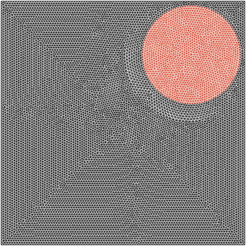
A body fitted triangular grid arrangement (as shown in Figure 3) is employed. The grid size is decided after conducting a rigorous grid independence test (details are provided in the ‘Results and Discussion’ section).

Figure 3. A schematic representation of the grids for a particular position of the intrusion.

Conservation equation for temperature T at a cell q after discretization can be written as

(4) $a_q{T}_q=\sum _{\mathrm{n}\mathrm{b}}{a}_{\mathrm{n}\mathrm{b}}{T}_{\mathrm{n}\mathrm{b}}+b$(4)

In this equation, a_q is the center coefficient, a_nb are the influence coefficients for the neighboring cells, and b is the contribution of the constant part of the source term S_c in S = S_c + S_qT and of the boundary conditions. In Equation (4),

(5) $a_q=\sum _{\mathrm{n}\mathrm{b}}{a}_{\mathrm{n}\mathrm{b}}-S_q$(5)

The imbalance in Equation (4) summed over all the computational cells q is denoted by the residual R^T which is computed by pressure-based solver as

(6) $R^T=\sum _{\mathrm{c}\mathrm{e}\mathrm{l}\mathrm{l}\mathrm{s}q}\left|\sum _{\mathrm{n}\mathrm{b}}{a}_{\mathrm{n}\mathrm{b}}{T}_{\mathrm{n}\mathrm{b}}+b-a_q{T}_q\right|$(6)

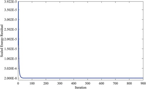
This is referred to as the ‘unscaled’ residual. It is difficult to judge convergence by examining the residuals defined by Equation (6), since no scaling is employed. A scaling factor (representative of the heat flow rate through the domain) is used to scale the residual. This ‘scaled’ energy residual is defined as

(7) ${\bar{R}}^T=\frac{\sum _{\mathrm{c}\mathrm{e}\mathrm{l}\mathrm{l}\mathrm{s}q}\left|\sum _{\mathrm{n}\mathrm{b}}{a}_{\mathrm{n}\mathrm{b}}{T}_{\mathrm{n}\mathrm{b}}+b-a_q{T}_q\right|}{\sum _{\mathrm{c}\mathrm{e}\mathrm{l}\mathrm{l}\mathrm{s}q}\left|a_q{T}_q\right|}$(7)

The scaled residual is a more appropriate indicator of convergence. Here, the scaled residuals are computed at each iteration. Once all these scaled residuals fall below a prescribed value, it is assumed that convergence is reached. In this study, a fixed value of 2 × 10⁻⁸ for the scaled energy residual is chosen as the prescribed value of convergence. The plot of scaled residual with number of iterations is shown in Figure 4.

Figure 4. Plot of scaled energy residuals with iteration number.

Reverse Problem (Prediction Methodology)

To predict the position of the intrusion, computational codes are developed (using ‘C’ programming language) adopting two different approaches: first one is based on the feed-forward NN with parametric study and second one is based on the GA-tuned feed-forward NN. In both cases, connecting weights are optimized through back-propagation (BP) algorithm. The problem here is to predict the position of the intrusion within the slab by knowing the temperature profile at the bottom wall of the slab. Temperature profile is collected in terms of temperatures at 11 specified positions (in a regular interval) along the bottom wall. These 11 temperatures are the inputs of the NN, and x and y coordinates of the intrusion-center are considered as the outputs of the network. Therefore, the network has 11 neurons for 11 inputs in the input layer and two neurons for two outputs in the output layer (Figure 5). Only one hidden layer is considered here. The neurons of input layer are assumed to have linear transfer function, whereas neurons of hidden and output layers have tan-sigmoid transfer functions.

Figure 5. Schematic representation of the adopted multi-layer feed-forward NN.

To update and to obtain the optimized weights of the network (which can predict the outputs with the minimum deviation) BP algorithm (Ghosh et al. 2012) is utilized. Besides the connecting weights, the performance of the NN depends on some other parameters, namely learning rate (η), momentum factor (α), slope of linear transfer function of input layer ($a_I$), transfer function coefficients of the hidden ($a_H$) and output ($a_O$) layers and number of neurons in the hidden layer ($N_H$). To predict the position of the intrusion more accurately, these parameters have to be optimized. To do this, two different approaches have been followed, as explained below.

Approach 1: A Thorough Parametric Study

In this approach, an attempt is made to optimize the said parameters (η, α, $a_I$, $a_H$, and $N_H$) through a parametric study. Here, only one parameter is varied at a time keeping the others fixed. Value of the parameter for which the percentage deviation in predictions comes out to be the minimum is selected as the optimum value of the same. Other parameters are optimized one after another in steps in the same way. Thus, in the present approach, optimal values of NN parameters are selected in stages. Computational codes are developed for NN using ‘C’ programming language.

Approach 2: A Combined GA-NN

Here, a GA (Ghosh et al. 2013) is used to optimize the NN parameters, namely η, α, $a_I$, $a_H$, $a_O$ and $N_H$. The GA starts with a randomly generated population of possible solutions (i.e., different set of the NN parameters). Members of the population are called GA-string (chromosome), which carries the information of those NN parameters ($a_I$, $a_H$, $a_O$, α, η, N_H), used to form the network. NN parameters are coded in the GA-string using binary coding. The field size for each of the variables is chosen as 14. As there are six variables, the total length of a chromosome becomes equal to 84. Thus, a representative GA-string looks like as follows:

Table

$a_I$	$a_H$	$a_O$	α	η	NH
01101111110000	01011001100011	00001110110110	01101111110100	00101010111011	11000111111110

The first 14 bits, that is, 01101111110000 yield the decoded value (DV) as 0 ×2¹³ + 1 ×2¹² + 1 ×2¹¹ + 0 ×2¹⁰ + 1 ×2⁹ + 1 ×2⁸ + 1 ×2⁷ + 1 ×2⁶ + 1 ×2⁵ + 1 ×2⁴ + 0 ×2³ + 0 ×2² + 0 ×2¹ + 0 ×2° = 7152. The real value of $a_I$is determined following the linear mapping rule as given below.

(8) $a_I=a_{I,min}+\frac{a_{I,max}-a_{I,min}}{2^{fieldsize}-1}\times DV$(8)

The real values of other variables are calculated following the similar procedure. After determining the real values of the parameters from the GA-string the NN is formed. Once the network is formed, a BP algorithm is activated to optimize the weights of the network, so that it can predict the outputs with minimum error. After updating the weights, percentage error/deviation in prediction is calculated and assigned as the fitness value of the corresponding string. The fitness values of all the other members of the population are calculated in the same way. The population become enriched by using the ‘reproduction’ (to select the better solutions from the present population pool for the next operations), ‘crossover’ (to exchange properties between two parents’ chromosomes) and ‘mutation’ (to introduce diversity in the solution space and to avoid convergence in the local optima) operators in each generation. A large number of generations are used to get the optimum globally enriched solutions. ‘Tournament selection’ scheme is used as the ‘reproduction operator’ and ‘uniform crossover’ is utilized as the ‘crossover’ operator in the present study. Figure 6 shows the schematic representation of the hybrid GA-tuned NN approach. Computational codes are developed for GA, NN as well as for the hybridization between NN and GA using ‘C’ programming language.

Figure 6. A schematic showing the proposed GA-tuned NN methodology (approach 2).

Results and Discussion

At first, detail about the grid independence test is provided. Then results obtained through the developed approaches to predict the intrusion location (center of the intrusion) within the slab are presented and discussed.

Grid Independence Test

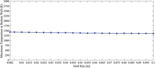
A triangular mesh is considered for the forward problem. The size of the grid is varied keeping the other parameters fixed. Mesh file is generated corresponding to each of the value of grid size, and then temperature profile at the bottom wall is evaluated through numerical simulation (as described above) corresponding to each of these mesh files. Temperature profile at bottom wall is plotted for each of the grid size as shown in Figure 7. The maximum temperature at the bottom wall is evaluated corresponding to each of the grid size. A plot is made between the maximum temperature (at bottom wall) and the corresponding grid size (as shown in Figure 8) to capture the variation of maximum temperature (at bottom wall) with grid size. There is a range of grid size, in which no significant changes are found in the temperature profiles (in Figure 7) or in the maximum temperature in the bottom wall (in Figure 8). Then, a value of grid size lying within this range is chosen as the grid size during meshing for data generation (Training and Test data). During grid independent test, intrusion-center is placed at the center of the slab (point [0, 0] with respect to the coordinate system as described in the ‘Problem Formulations’ section) and radius of the intrusion is considered as 0.2 m. Through the grid independent test, the grid size is selected as 0.01 m for the rest of the study.

Figure 7. Temperature profile at the bottom wall of the square slab for different grid sizes (center of the intrusion is placed at the center of the slab; r = 0.2 m).

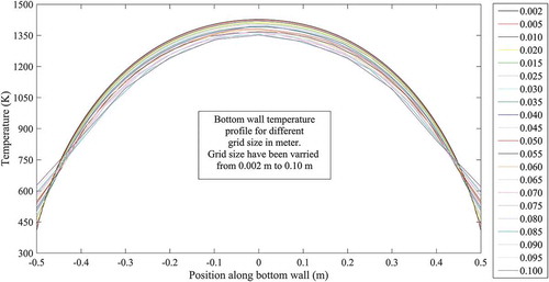
Figure 8. Variations of maximum temperature at bottom wall with grid size (position of the center of the intrusion is chosen at the center of the slab; radius of the intrusion is 0.2 m).

Prediction of the Intrusion-Position

The radius of the circular copper intrusion is considered as 0.2 m, and the data are collected by varying the position of the circular intrusion throughout the square slab. Data are collected for 841 different positions of the intrusion. The temperature profiles at the bottom wall for seven different positions of the intrusion are shown in Figure 9. It is clear from Figure 9 that the temperature profiles at the bottom wall are very much responsive to the intrusion-position within the bulk. Therefore, it is possible to estimate or predict the intrusion-position by knowing the temperature profile at the bottom wall of the slab.

Figure 9. Temperature profiles at the bottom wall of the square slab for seven different positions of the circular intrusion with radius 0.2 m.

Prediction of Intrusion-Position Using Approach 1

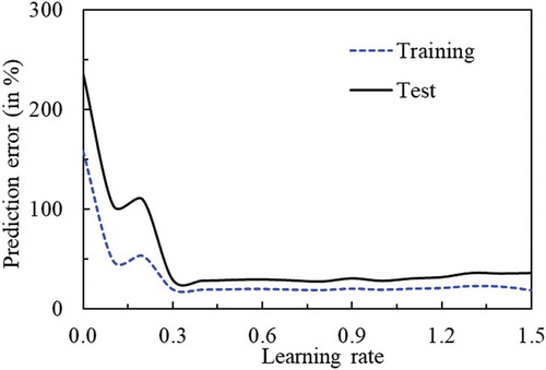
In approach 1, optimum values of the NN parameters, namely learning rate (η), momentum factor (α), slope of linear transfer function in input layer ($a_I$), transfer function coefficient of the hidden ($a_H$) and output layer ($a_O$) and number of neurons in the hidden layer ($N_H$) are optimized in stages. One parameter is varied at a time from its minimum possible value to maximum allowable value keeping other parameters fixed to decide the optimal value of that particular parameter. Value of the parameter for which percentage error in prediction becomes minimum is selected as the optimum one. The percentage error in prediction is defined as

(9) $\mathrm{P}\mathrm{e}\mathrm{r}\mathrm{c}\mathrm{e}\mathrm{n}\mathrm{t}\mathrm{a}\mathrm{g}\mathrm{e}\mathrm{E}\mathrm{r}\mathrm{r}\mathrm{o}\mathrm{r}\mathrm{i}\mathrm{n}\mathrm{P}\mathrm{r}\mathrm{e}\mathrm{d}\mathrm{i}\mathrm{c}\mathrm{t}\mathrm{i}\mathrm{o}\mathrm{n}=\left[\frac{1}{Z}\sum _{z=1}^{z=Z}\left\{\frac{1}{K}\sum _{k=1}^K\left(\frac{\left|T_{Ozk}-O_{Ozk}\right|}{T_{Ozk}}\right)\right\}\right]\times 100.0,$(9)

where, Z represents the numbers of training/test scenarios and K denotes the number of outputs. T_Ozk indicates the target output for the k-th output neuron corresponding to z-th scenario and O_Ozk denotes the network predicted value of the same. Once one parameter is optimized, it is kept fixed for the rest of the parametric study. To determine optimal values of the other parameters, similar studies are carried out. During optimization of $N_H$ using parametric study, allowable maximum value of $N_H$ is decided as explained below. There are 11 input neurons and 2 output neurons in the input and output layers of the NN, respectively. If the value of $N_H$ is x, then the total number of connecting weights in the network becomes equal to (11x + 2x). Therefore, (11x + 2x) should be either less than or equal to the number of training scenarios (Z), i.e., (11x + 2x) ≤ Z or x ≤ (Z/13). The number of training scenarios, Z, means, Z number of input–output data are used during training to update and optimize the weights. Therefore, the range of search for N_H becomes 0 < N_H ≤ (Z/13). However, the number of neuron cannot be a fraction. The parametric study for learning rate (η) is shown in Figure 10. This figure shows the variation of percentage error in prediction with learning rate (keeping other parameters fixed) using the training and test data. The lowest value of the percentage error in prediction is found at η = 0.8. Therefore, the optimum value of learning rate is considered as 0.8. For the others, parametric studies are performed in the same way. The optimum values of the NN parameters obtained through parametric study are as follows: η = 0.8, α = 0.47, $a_I$= 1.1, $a_H$ = 1.0, $a_O$ = 0.97 and $N_H$ = 11.

Figure 10. Variations of prediction error (%) with learning rate keeping other parameters fixed.

The performance of the optimized NN (using parametric study and BP algorithm) is tested with the help of test data. The average test error in prediction is found as 18.95%. The distributions of test error in prediction along the line x = 0.0, obtained using approach 1, are shown in Figure 11. In this figure, center of each circle denotes the exact position of the intrusion-center and the radius of the circle represents the prediction error around that position. The radius of the circle is calculated as

(10) $\mathrm{R}\mathrm{a}\mathrm{d}\mathrm{i}\mathrm{u}\mathrm{s}=\sqrt{{\left(x_e-x_p\right)}^2+{\left(y_e-y_p\right)}^2},$(10)

Figure 11. Distribution of test errors in prediction along the line x = 0 using approach 1.

where $\left(x_e,y_e\right)$ indicates the coordinate of the exact position of the intrusion-center and $\left(x_p,y_p\right)$ represents the coordinate of the predicted position of the intrusion-center. Therefore, the radius of error circle becomes zero, if the predicted position perfectly matches with the exact position.

The predicted positions of the intrusion using approach 1 are validated or tested by performing numerical simulations of the forward problem considering intrusion at the predicted position. Validations/tests are made by comparing the bottom-wall temperature profile when intrusion is in the exact position with that when intrusion is in the predicted position. Figure 12 shows these comparisons at six different locations along the line x = 0.0. For each case, red curve represents the temperature profile with original position of the intrusion and black curve indicates the temperature profile with the predicted position of the intrusion. In each case, the original position of the intrusion is mentioned in Figure 12. For a better realization, temperatures along bottom wall with predicted position of the intrusion are plotted against that with actual position of the intrusion. These plots are shown in Figure 13 for six different locations along the line x = 0.0. Here the plots are made by considering wall temperatures with actual position along the axis of abscissas (horizontal axis) and wall temperatures with predicted position along the axis of ordinates (vertical axis). Deviations of the predicted position from the original position can be judged by the distance of the plotted points from the line with slope 1 (tan 45°). Points situated on the line with slope 1, represent the perfect matching between the predicted and original positions of the intrusion. Validation in terms of comparisons between the temperature contours with original and predicted (using approach 1) position of the intrusion are shown in Figure 14.

Figure 12. Validations by comparing the bottom-wall temperature profile when intrusion is in the exact position with that when intrusion is in the predicted (using approach 1) position.

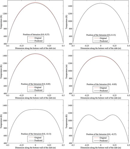
Figure 13. Validation/test in terms of plots between the temperatures along bottom wall with predicted (using approach 1) and exact position of the intrusion (along x = 0.0).

Figure 14. Validation/test in terms of comparison between the temperature contours with exact and predicted (through approach 1) position of the intrusion (along x = 0.0).

Prediction of Intrusion-Position Using Approach 2

Here, the optimum set of NN parameters are obtained using GA. Figure 15 shows the variation of the best GA-fitness value (% error in prediction) with the numbers of generations during GA-run. It is important to note that after 23 generations, there is no change in the value of the best GA-fitness value. This study confirms the convergence of the GA-search. After using the optimum set of NN parameters obtained through GA, the variation of percentage error in prediction with the number of iterations during training using BP algorithm for weights updation/optimization is shown in Figure 16. The performance of the optimized NN (using GA and BP algorithm) is tested with the help of test data. The obtained percentage errors in prediction using approach 2 in different regions of the bulk are shown in Table 1. The distributions of the test errors in prediction using approach 2 in different regions of the bulk are shown in Figure 17. As described in the previous sub-section (using Equation 10), the center of each circle denotes the exact position of the center of the intrusion and the radius of that represents the error in prediction around that position. From Figure 17, it is generally observed that the intrusion-positions in the lower half of the bulk are more accurately predicted compare to that in the upper half.

Table 1. Test errors in prediction (%) for different regions of the bulk using approach 2.

Case	Average test error in prediction (%)
Intrusion moves along x = −0.28	16.22
Intrusion moves along x = −0.14	18.81
Intrusion moves along x = −0.06	13.25
Intrusion moves along x = 0.00	13.67
Intrusion moves along x = 0.06	11.70
Intrusion moves along x = 0.14	15.67
Intrusion moves along x = 0.28	18.17

Figure 15. GA-fitness (% error in prediction) versus maximum number of generations.

Figure 16. Variation of NN training error (in percent) with the number of iterations of BP algorithm during weights updation/optimization.

Figure 17. Distribution of test errors in prediction in different regions of the bulk using approach 2.

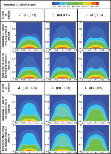
The predicted positions of the intrusion using approach 2 are also validated or tested (just like using approach 1) by performing numerical simulations of the forward problem considering intrusion at the predicted position. At first, predicted positions are validated/tested along the line x = −0.28 by making comparisons between the bottom-wall temperature profiles with actual and predicted (using approach 2) positions of the intrusion as shown in Figure 18. Validation/test along the line x = −0.14 are made by making plots between the bottom-wall temperatures with actual and predicted (by approach 2) position of the intrusion where temperatures for actual position are considered along the axis of abscissas and temperatures for predicted positions are considered along the axis of ordinates. These plots are shown in Figure 19. Validated and tested results in terms of comparisons between the temperature contours with actual and predicted position of the intrusion along the line x = −0.06 are shown in Figure 20. To validate/test the results along the line x = 0, plots are made by considering temperatures of bottom wall along the axis of abscissas for actual positions and along the axis of ordinates for predicted positions of the intrusion as shown in Figure 21. As validation/test (using approach 2) along line, x = 0.06, Figure 22 shows the comparisons between the temperature profiles at bottom wall with actual and predicted positions of the intrusion. To validate/test the results, temperature contours for actual positions of intrusion are compared with that for predicted positions of the intrusion along the line x = 0.1, as shown in Figure 23. Along x = 0.28, validated/tested results in terms of comparisons between the temperature profiles at bottom wall for actual and predicted (using approach 2) positions of the intrusion are shown in Figure 24.

Figure 18. Validation/test in terms of comparisons between the temperature profiles at bottom wall with exact and predicted (through approach 2) position of the intrusion (along x = –0.28).

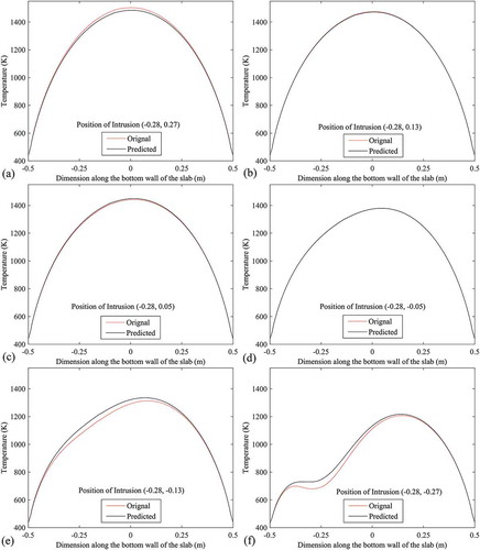
Figure 19. Validation/test in terms of plots between the temperatures along bottom wall with predicted (using approach 2) and exact position of the intrusion (along x = –0.14).

Figure 20. Validation/test in terms of comparison between the temperature contours with exact and predicted (through approach 2) position of the intrusion (along x = –0.06).

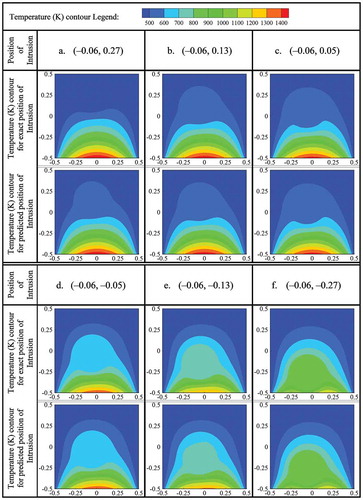
Figure 21. Validation/test in terms of plots between the temperatures along bottom wall with predicted (using approach 2) and exact position of the intrusion (along x = 0.0).

Figure 22. Validation/test in terms of comparisons between the temperature profiles at bottom wall with exact and predicted (using approach 2) positions of the intrusion (along x = 0.06).

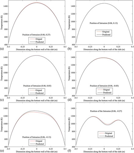
Figure 23. Validation/test in terms of comparisons between the temperature contours with actual and predicted (using approach 2) positions of the intrusion (along x = 0.14).

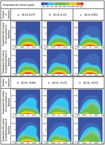
Figure 24. Validation/test in terms of comparisons between the temperature profiles at bottom wall with actual and predicted (using approach 2) positions of the intrusion (along x = 0.28).

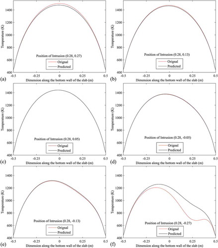
By analyzing Figures 17–24, it is found that the bottom-wall temperature profile is very sensitive to the intrusion-position and this sensitivity increases as it (intrusion) moves toward (become closer to the) bottom wall. As a result, for a very long distance of the intrusion from bottom wall, very similar bottom-wall temperature profiles (for the predicted and original position) may be obtained even though the deflection of predicted position from the original position is large. Again, when the intrusion is very close to the bottom wall, large deviation between the bottom-wall temperature profiles (with predicted and original position of intrusion) may be found even though the predicted position is very close to the original position. These two findings are clearly visible if one compare Figures 17(a) and 18 or Figures 17(b) and 19 or Figures 17(e) and 22 or Figures 17(g) and 24, separately. From Figures 20 and 23, again it is found that deviation between the original and predicted position of intrusion (in terms of temperature contour) is more in the upper half of the slab compare to the lower half.

Concluding Remarks

Methodologies have been developed to inspect the heterogeneity in a homogeneous bulk using numerical analysis of 2D heat conduction and indigenously bred hybrid computational intelligence. Problem is defined as to predict the location of a circular intrusion of other material within a square homogenous bulk from some known temperature profile collected at the bottom surface of the bulk. The data (temperature history along bottom surface of the bulk for different positions of the intrusion) have been numerically evaluated by the forward calculations using commercial CFD software (Fluent) in a fully automated way by indigenously developed algorithm using ‘C’ programming language. Two approaches have been developed using multi-layer feed-forward NN with BP algorithm to solve the reverse (prediction) problem. In approach 1, the NN parameters have been optimized through a thorough parametric study by varying them one after another in stages. In approach 2, the NN parameters have been optimized simultaneously by utilizing one global optimizer namely GA. NN parameters together with the connecting weights involves a large number of variables, a GA alone may not be sufficient to optimize them together due to its inherent permutation problem. Realizing this fact, the task of updating the connecting weights of NN has been given to a local optimizer like BP algorithm. The performances of the developed approaches to predict the intrusion-position have been tested and validated in multiple way.

Temperature profile at the bottom surface has been found very sensitive to the intrusion-position within the bulk and this sensitivity increases as it become closer to the bottom surface. As a result, intrusion-position can be predicted more accurately when lies in the lower half of the bulk compare to that in the upper half. When intrusion is very far from the bottom surface, almost identical bottom-wall temperature profiles (for the predicted and original position) may be found even for a large deflection of the predicted position from the original position. Again, for a very close position of the intrusion (from bottom surface), large diversion between the bottom-wall temperature profiles (with predicted and original position of intrusion) may be obtained even for a very small deviation of the predicted position from the original position.

Comparisons between the performances of approaches 1 and 2 reveal that approach 2 performs in better way to predict the intrusion-position within the bulk. It is found so due to the fact that in approach 1, appropriate values of NN parameters are determined in stages, whereas in approach 2, the said NN parameters are optimized concurrently using one global optimizer namely GA. In this approach, global search capability of the GA is coupled with the local search power of BP algorithm. Thus, a hybrid optimization scheme is implemented in approach 2 and consequently, it performs in better way compare to the other. This proposal is found to be a reasonably efficient tool for prediction in heat conduction problems.

The shape and size of the intrusion were kept fixed during development of the methodologies for prediction. Therefore, they can estimate the location of intrusion only. By varying the shape and size of the intrusion, the methodology can be modified further to estimate the shape and size of the intrusion or can be extended further to estimate the position together with the shape and size of intrusion. Proposed hybrid approach can be modified and extended further to solve other prediction problems in conduction or in another mode of heat transfer.

References

- Agnelli, J. P., A. A. Barrea, and C. V. Turner. 2011. Tumor location and parameter estimation by thermography. Mathematical & Computer Modelling 53:1527–34. doi:10.1016/j.mcm.2010.04.003.
- Ahmadi, I., N. Sheikhy, M. M. Aghdam, and S. S. Nourazar. 2010. A new local meshless method for steady-state heat conduction in heterogeneous materials. Engineering Analysis with Boundary Elements 34:1105–12. doi:10.1016/j.enganabound.2010.06.012.
- Amri, A., A. Saidane, and S. Pulko. 2011. Thermal analysis of a three-dimensional breast model with embedded tumour using the transmission line matrix (TLM) method. Computers in Biology and Medicine 41:76–86. doi:10.1016/j.compbiomed.2010.12.002.
- Ang, W. T., and B. I. Yun. 2011. A complex variable boundary element method for axisymmetric heat conduction in a nonhomogeneous solid. Applied Mathematics and Computation 218:2225–36. doi:10.1016/j.amc.2011.07.039.
- Ang, W. T., and D. L. Clements. 2010. Nonlinear heat equation for nonhomogeneous anisotropic materials: A dual-reciprocity boundary element solution. Numerical Methods for Partial Differential Equations 26:771–84. doi:10.1002/num.20452.
- Ghosh, S., D. K. Pratihar, B. Maiti, and P. K. Das. 2012. Identification of flow regimes using conductivity probe signals and neural networks for counter-current gas–liquid two-phase flow. Chemical Engineering Science 84:417–36. doi:10.1016/j.ces.2012.08.042
- Ghosh, S., D. K. Pratihar, B. Maiti, and P. K. Das. 2013. Automatic classification of vertical counter-current two-phase flow by capturing hydrodynamic characteristics through objective descriptions. International Journal of Multiphase Flow 52:102–20. doi:10.1016/j.ijmultiphaseflow.2012.12.007.
- Itou, S. 2004. Thermal stresses around a crack in the nonhomogeneous interfacial layer between two dissimilar elastic half-planes. International Journal of Solids and Structures 41:923–45. doi:10.1016/j.ijsolstr.2003.09.056.
- Kassab, A. J., and E. A. Divo. 1996. A generalized boundary integral equation for isotropic heat conduction with spatially varying thermal conductivity. Engineering Analysis with Boundary Elements 18:273–86. doi:10.1016/S0955-7997(96)00057-4.
- Khor, K. A., and Y. W. Gu. 2000. Thermal properties of plasma-sprayed functionally graded thermal barrier coatings. Thin Solid Films 372:104–13. doi:10.1016/S0040-6090(00)01024-5.
- Ng, E. Y. K. 2009. A review of thermography as promising non-invasive detection modality for breast tumor. International Journal of Thermal Sciences 48:849–59. doi:10.1016/j.ijthermalsci.2008.06.015.
- Ng, E. Y. K., and E. C. Kee. 2008. Advanced integrated technique in breast cancer thermography. Journal of Medical Engineering & Technology 32:103–14. doi:10.1080/03091900600562040.
- Ng, E. Y. K., and S. C. Fok. 2003. A framework for early discovery of breast tumor using thermography with artificial neural network. The Breast Journal 9:341–43. doi:10.1046/j.1524-4741.2003.09425.x.
- Shiah, Y. C., and Y. X. Shi. 2006a. Anisotropic heat conduction across an interface crack/defect filled with a thin interstitial medium. Engineering Analysis with Boundary Elements 30:325–37. doi:10.1016/j.enganabound.2006.01.012.
- Shiah, Y. C., and Y. X. Shi. 2006b. Heat conduction across thermal barrier coatings of anisotropic substrates. International Communications in Heat and Mass Transfer 33:827–35. doi:10.1016/j.icheatmasstransfer.2006.04.006.
- Song, C., V. Appleyard, K. Murray, T. Frank, W. Sibbett, A. Cuschieri, and A. Thompson. 2007. Thermographic assessment of tumor growth in mouse xenografts. International Journal of Cancer 121:1055–58. doi:10.1002/ijc.22808.
- Tan, T. Z., C. Quek, G. S. Ng, and E. Y. K. Ng. 2007. A novel cognitive interpretation of breast cancer thermography with complementary learning fuzzy neural memory structure. Expert Systems with Applications 33:652–66. doi:10.1016/j.eswa.2006.06.012.
- Yun, B. I., and W. T. Ang. 2010. A dual-reciprocity boundary element approach for axisymmetric nonlinear time-dependent heat conduction in a nonhomogeneous solid. Engineering Analysis with Boundary Elements 34:697–706. doi:10.1016/j.enganabound.2010.03.013.