Assessing the Explanatory Power of Dwelling Condition in Automated Valuation Models

Abstract

This study investigates the role of dwelling-condition attributes in automated valuation models (AVMs) by utilizing detailed dwelling-condition assessment reports in Norway. A hedonic linear regression model, a gradient boosted decision tree, and a support vector machine were trained and evaluated to predict the sale price of dwellings in three urban regions. The study aims to evaluate the explanatory power of condition attributes in AVMs through a comparison of predictive performance with and without these attributes. The results indicate that the inclusion of condition attributes significantly improves the accuracy of all models across all regions. Furthermore, the models show consistent results regarding which condition attributes are important and their relationship to the price. The study finds that the condition of the bathroom has a high impact on the price, while the condition of doors, roof, and exterior extensions has a low impact. The study concludes that dwelling condition holds explanatory power in both linear and nonlinear AVMs, which can benefit researchers, practitioners, and homeowners looking to renovate. The findings highlight the importance of including detailed dwelling-condition attributes in AVMs and provide insights into the valuation of different aspects of a dwelling.

Keywords:

• Forecasting
• explainable AI
• dwelling condition
• assessment reports
• housing valuation

JEL CLASSIFICATIONS:

• C55
• R21
• R31

Introduction

Real estate is an important class of assets that constitutes a large part of any country’s economy and involves a wide range of stakeholders. Whether to be used in a purchasing decision, to determine the appropriate size of a mortgage, or to estimate taxable wealth, accurate valuations of real estate properties are of interest to individuals, banks, and governments alike. Historically, real estate valuation methods involve single-property valuations, which rely to a great extent on the appraiser’s subjective experience and judgment. Due to their objective and systematic valuations, in addition to their ability to perform mass appraisals in a time- and cost-efficient manner, automated valuation models (AVMs) have gained popularity in recent years. AVMs have obtained a central role in the growing proptech industry and among iBuy companies, where renovation plays an important role (Anderson et al., 2023; Harrison et al., 2023; Helgaker et al., 2022; Seiler & Yang, 2023). AVMs typically rely on regression models trained on historical sales data that attempt to capture the relationship between a property’s characteristics and its price. Some commonly considered property characteristics include location; structural information, such as size or number of rooms;, and neighborhood factors, such as air pollution and crime rate. However, little research has been dedicated to assessing the explanatory power of a dwelling’s condition.

This study aims to bridge this gap in the literature and assess the explanatory power of a dwelling’s condition in AVMs. To achieve this, a hedonic linear regression model, a gradient boosted decision tree, and a support vector machine (SVM) are trained using the sales data for dwellings in Oslo and its surroundings, Bergen, and Trondheim, three urban regions in Norway. To the best of the authors’ knowledge, this is the first study that aims to assess the explanatory power of condition attributes in both linear and nonlinear AVMs. Furthermore, the data used are unique, in terms of both the granularity of the condition assessments and their close proximity to the time of sale. Knowledge about the impact of dwelling condition on the sale price can be of value for two reasons. First, it can help researchers and practitioners increase the accuracy of AVMs. Second, it may aid homeowners in assessing the profitability of renovating various aspects of the dwelling.

This study uses data provided by the Norwegian proptech start-up Vendu AI. The data contain assessments of the condition of dwellings being put up for sale, in the form of reports written by assessors. This study utilizes data sets covering three regions in Norway: 6651 dwellings in Oslo and its surroundings, 2975 dwellings in Bergen, and 1677 dwellings in Trondheim. Attributes describing the size, location, build year, selling year, and building type are included, in addition to attributes describing the condition of a range of checkpoints within the dwelling, such as the kitchen, bathroom, and building structure.

To assess the explanatory power of dwelling condition in AVMs, the models are trained with and without condition attributes, and their predictive performance is recorded and compared. The data are split into a training set and a test set, so that the out-of-sample predictive performance can be accurately assessed. The root mean squared error (RMSE), mean percentage error (MPE), mean absolute percentage error (MAPE), and percentage of prices predicted within 10% and 50% of the actual selling price are used to assess the performance. Finally, the models are interpreted to analyze the determined relationship between condition and price.

The inclusion of dwelling condition resulted in accuracy improvements in all three regression models. All models benefited similarly in magnitude, and the accuracy gain was consistent across the three regions. The models were also consistent in terms of which condition attributes ranked high in importance and the relationship between these attributes and the price. The combination of increased predictive accuracy and consistency in model interpretations leads us to conclude that dwelling condition provides explanatory power in AVMs. However, this explanatory power varies between condition categories. Across all models and regions, the condition of the bathroom has a high impact on the price, while the condition of the doors, roof, and exterior extensions has a low impact.

This paper is structured as follows: “Related Literature Review” section reviews related literature on real estate valuation, covering traditional and modern machine learning approaches and previous work exploring the relationship between dwelling condition and sale price; “Real Estate Market in Norway” section provides relevant background on the housing markets in the three regions, as well as an introduction to the structure of the condition reports utilized in the study; “Data” section presents a statistical description of the data; “Methodology” section describes the methodology, including a theoretical introduction to the models used; “Results and Discussion” section presents and discusses the results; and “Conclusion” section concludes the study, summarizing the most important findings.

Related Literature Review

AVM Approaches

A wide variety of techniques have been applied to the automatic prediction of dwelling prices, but the oldest and most prominent is the linear regression model. Lin- ear regression models in AVMs are based on the theory of the hedonic price function, as outlined by Rosen (1974). By breaking down the property into its characteristics, the estimated coefficients of the linear regression function represent the implicit marginal price of each characteristic and provide an economic interpretation of their value. The predictive accuracy of linear regression models in AVMs has been thoroughly examined, and researchers frequently use them as a baseline for comparisons to other models (Antipov & Pokryshevskaya, 2012; Do & Grudnitski, 1992; Kok et al., 2017; Lam et al., 2009; Lin & Mohan, 2011; Marjan et al., 2018; Mimis et al., 2013; Nghiep & Al, 2001).

The support vector machine (SVM; Cortes & Vapnik, 1995) is a machine learning approach that can outperform the linear regression model in terms of predictive accuracy. This superior performance is attributable to the SVM’s ability to efficiently capture nonlinear relationships, the relative ease of finding optimal values for its hyperparameters and the guarantee of a globally optimal model (Chen et al., 2017; Kontrimas & Verikas, 2011; Lam et al., 2009).

Another class of machine learning approach used in AVMs is the ensemble method, in which multiple models are trained and an aggregated output is used as the prediction. Ensemble methods that show promising results in terms of accurately predicting dwelling prices include random forests (Antipov & Pokryshevskaya, 2012; Dimopoulos et al., 2018; Marjan et al., 2018), boosting methods (Ho et al., 2021; Kok et al., 2017; Mayer et al., 2019), and stacking methods (Graczyk et al., 2010; Kontrimas & Verikas, 2011).

Dwelling Condition

Most real estate research focuses on methods of enhancing the predictive accuracy of AVMs, and few conclusions have been drawn regarding the explanatory power of dwelling condition. Recent examples of studies considering dwelling condition include Doumpos et al. (2020), Renigier-Biłozor et al. (2019), and Helbich and Griffith (2016), but the dwelling attributes considered are general and few, with no explicit conclusions drawn regarding their explanatory power.

One of the first studies to attempt to establish the economic value of dwelling condition was Kain and Quigley (1970). That study uses five categories to describe the condition of a dwelling. The categories are determined by factor analysis of 39 initial variables, which are derived partly from surveys asking homeowners to assess the quality of various aspects of their property and partly from city building inspectors’ assessments of neighborhood factors. When regressed against the sale price, three of the five categories were deemed significant, indicating that homeowners were willing to pay for higher quality.

Instead of relying on a homeowner’s subjective assessment of dwelling condition, Ooi et al. (2014) use a standardized metric assessed by professionals. The Construction Quality Assessment System (CONQUAS) is used in Singapore to assess three categories describing a property’s condition. When regressed against price, dwellings with a better CONQUAS score were found to command a higher price. More recently, Mathur (2019) considers dwelling condition based on construction quality and level of maintenance, measured by standardized scales defined by the local tax assessor. Both factors were found to significantly and positively affect the price.

Overall, the studies agree that dwelling condition has a statistically significant relationship to dwelling price, and dwellings in better condition typically command higher prices. However, these studies are lacking in some regards. First, the level of detail in the descriptive attributes is low. Second, there is often a large gap between the time of assessment and the time of sale. Third, the studies employ only linear regression models and draw no conclusions regarding the explanatory power of condition attributes of predicting dwelling prices. This study extends the literature by examining the impact of dwelling condition, using both linear and nonlinear models in the framework of AVMs.

Real Estate Market in Norway

The explanatory power of dwelling condition in AVMs is examined using dwellings from three data sets covering urban regions in Norway. This section presents information regarding the housing markets in these regions. Maps of the regions are provided in Appendix D. A more detailed description is provided for the housing market in Oslo and its surroundings, which is this study’s main area of focus. An explanation of the property transaction process and the condition reports utilized in the study is also provided.

The Property Market in Oslo and Surroundings

The data set covering Oslo and its surroundings includes dwellings located in the city of Oslo and in the five surrounding municipalities of Bærum, Drammen, Asker, Lillestrøm, and Lørenskog. This area will simply be referred to as Oslo for the remainder of the study. The decision to include additional municipalities was motivated primarily by data availability. Additionally, the surrounding municipalities are densely populated urban areas that are part of the Oslo Region Alliance, a group of municipalities that consider the capital their natural center.¹ The city of Oslo is the capital of Norway and had a total population of 693,494 as of January 1, 2020 (SSB, 2021). The combined population of Bærum, Drammen, Asker, Lillestrøm, and Lørenskog was 446,964 as of January 1, 2019 (Mæhlum, 2020).

The average square meter price in the city of Oslo was NOK 77,342 in 2019 (Oslo Municipality, 2021). The square meter prices were somewhat lower in the surrounding municipalities: NOK 40,457 in Drammen, NOK 49,659 in Lillestrøm, NOK 64,062 in Bærum, NOK 45,128 in Asker, and NOK 51,970 in Lørenskog (Krogsveen, 2021). All locations in the Oslo data set experienced a substantial price increase over the last decade. The city of Oslo had an increase of 85% between 2010 and 2020, while the other five municipalities in Viken County had an increase of between 68% and 81% within the same period (Krogsveen, 2021).

The Property Market in Bergen and Trondheim

The other regions covered in the study are the municipalities of Bergen and Trondheim, the second and third largest cities in Norway. Bergen lies in Vestland County and has a population of 283,929 (Bergen Municipality, 2020). Trondheim lies in Trøndelag County and has a population of 207,595 (Trondheim Municipality, 2020). The square meter prices in both regions ranged from approximately NOK 30,000 to NOK 50,000 in 2020 (Krogsveen, 2021), indicating a generally lower price level than in Oslo. It is also worth noting that Bergen and Trondheim have significantly fewer administrative districts than to Oslo.

Property Transaction Procedure and Condition Report

The property sale process in Norway is characterized as an English auction, in which the price is determined in a near-perfect bidding context (Olaussen et al., 2017). This, coupled with the fact that nonprofessional buyers and sellers dominate the Norwegian housing market, makes it highly suitable for studies of property pricing in general (Oust et al., 2020). The sale process in Norway typically goes as follows:

1. The seller hires a real estate agent and an assessor.

2. The assessor evaluates the technical condition of the property and compiles a report outlining the condition of the dwelling.

3. The real estate agent collects all available information, including the condition report; creates a sales report for potential buyers; and sets an asking price.

4. Potential buyers are given the opportunity to visit the property and assess it, typically through an announced public open house.

5. The real estate agent arranges an English auction. Bids are binding, and any bid accepted by the seller is a binding contract.

The condition report assesses various aspects of the home. It is a technical report covering everything from the condition of the floors to the quality of air circulation. It typically focuses on aspects of the dwelling that are difficult for buyers to assess during the showing and that often lead to conflicts between the seller and the buyer. The buyer is responsible for any deficiency in the dwelling as long as it has been reported before the bidding process. However, if it is not reported, the seller is often responsible.

Standards (2012, 2015) NS 3424 and NS 3600 exist to ensure consistency between condition reports. The standards describe what must be assessed and outline four levels describing the condition. This paper utilizes an inverted version of the scale originally used by the appraisers to address issues with data quality and to improve the interpretability of the results:²

1. Major faults: Reparations are required immediately.

2. Significant faults: Reparations are needed soon.

3. Small or moderate faults: No reparations are necessary, but there may be minor discrepancies.

Details on this modification are provided in “Data” section.

The dwelling condition levels were set by the appraisers based on previous sales, in line with the standards and independent of this research paper. Potetial home buyers were aware of these dwelling conditions at the time of sale.

Data

This study uses data provided by Vendu AI, a Norwegian proptech start-up. Vendu AI has access to data collected from two providers: Ambita and Norsk takst. Ambita is responsible for registering all property and land transactions in Norway and provides general sales data. Norsk takst is an industry organization for appraisers that provides condition reports. This section introduces the process of merging and cleaning the two data sets and provides a descriptive analysis of the final data. The final data set comprises dwellings in Oslo, Bergen, and Trondheim sold between 2016 and 2020.

Data Description

The format of the condition reports provided by Norsk takst requires preprocessing. The reports consist of a numerical score between zero and three, in addition to an accompanying descriptive text for checkpoints in the dwelling. These checkpoints are identified by a room number and a checkpoint number. Because not every checkpoint is relevant for every dwelling, the number of checkpoints with scores differs in each report. Consequently, the checkpoints cannot be used as attributes representing dwelling condition in the AVM. Furthermore, a visual inspection of checkpoint descriptions revealed that multiple checkpoints with scores of zero actually represented no score given. For this reason, all checkpoints with a score of zero were deemed corrupt and discarded.

A simple heuristic method was used to solve the problem of the varying number of checkpoints. Checkpoints were merged into categories, and the average score of the checkpoints was used to represent the condition of that category. Categories were defined by subjective judgments of which checkpoints could naturally be grouped to represent the condition of a given aspect of the dwelling. Reports with more than two scores missing after merging and averaging were discarded. For reports with two or fewer missing scores, the missing values were replaced by the average of the remaining categories. Finally, the scores were flipped so that a score of one corresponds to the lowest quality (TG3) and a score of three corresponds to the highest (TG1). This was done to make the results more intuitive. Table 1 provides an overview of the final condition attributes with their underlying checkpoints specified, as well as the noncondition attributes employed in the study.

Table 1. Overview of all attributes employed in the study.

Attribute	Type	Description
Building framework	Numeric	Condition of foundation, wall construction, and exterior facades
Plot	Numeric	Condition of plot drainage, retaining walls, driveways, gardens, and porch stairs
Windows	Numeric	Condition of all windows
Doors	Numeric	Condition of all doors
Roof	Numeric	Condition of roof construction and roofing
Exterior extensions	Numeric	Condition of balconies, railings, and terraces
Interior surfaces	Numeric	Condition of interior ceilings, walls, floors, stairs, and surfaces
Bathroom	Numeric	Condition of sanitary equipment, furnishings, air treatment systems, floors, ceilings, walls, wiring harnesses, plumbing, drains, membranes, and ceilings of bathrooms and wet rooms
Kitchen	Numeric	Condition of kitchen floors, walls, ceilings, equipment, furnishings, plumbing, sanitation, and air treatment
HVAC, sanitary	Numeric	Condition of heating systems, hot water systems, ventilation systems, air conditioning, and sanitation
Large plot	Binary	Indicates whether plot size is above 500 square meters
Build year	Numeric	Year of dwelling construction
Size	Numeric	Size of primary living space
Building type	Categorical	Apartment (A), townhouse (TH), detached house (DH), or semidetached house (SDH)
Region	Categorical	Administrative district of dwelling
Sale year	Numeric	Sale year of dwelling
Sale month	Numeric	Sale month of dwelling
Universal Transverse Mercator (UTM) coordinates	Numeric	UTM x- and y-coordinates for exact location of dwelling

Data Merging and Cleaning

The condition reports from Norsk takst and the general sales data from Ambita were merged by matching address information. The majority of apartments had insufficient address details to confidently match the condition report to the correct apartment unit, so they are mostly left out of the study. The data were cleaned by discarding any of the following dwellings:

• Dwellings with likely erroneous entries for price or size. Dwellings with an abnormally high or low square meter price were discarded.

• Dwellings with multiple matching condition assessments for the same date. This was done to ensure that the correct condition is matched with the correct price for all dwellings.

• Dwellings sold more than once within three months for more than double the first sale price.

• Dwellings lacking UTM coordinates.

Table 2 illustrates the process and shows the exact number of entries removed for each check.

Table 2. Number of dwellings removed at every step in the data cleaning process.

	Oslo	Bergen	Trondheim
Original size	7104	3308	1748
Abnormal size or price	47	18	12
Duplicated	400	315	59
Sold more than once	1	0	0
Missing location data	5	0	0
Final size	6651	2975	1677

The ten dwelling conditions were not chosen by us for this paper. However, the selection was implicitly determined by the data, since these ten building elements were the ones for which we were able to extract conditions for all the homes.

Data Exploration

This section presents an exploratory data analysis for the Oslo data set. For brevity, only Oslo is analyzed, since this is the largest data set and the main focus of the study.

Table 3 shows the sale year distribution of dwellings in Oslo, Bergen, and Trondheim. The majority of dwellings were sold in 2018, and only a small fraction were sold in 2020.

Table 3. Sale year distribution of dwellings in Oslo, Bergen, and Trondheim.

Sale year	Oslo	Bergen	Trondheim
2016	598 (8.99%)	534 (17.95%)	344 (20.51%)
2017	1906 (28.65%)	860 (28.91%)	454 (27.07%)
2018	2283 (34.33%)	896 (30.12%)	521 (31.07%)
2019	1825 (27.44%)	668 (22.45%)	346 (20.63%)
2020	39 (0.59%)	17 (0.57%)	12 (0.72%)

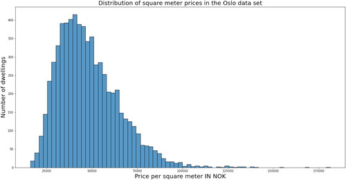
Figure 1 shows the distribution of the square meter price in NOK of dwellings in Oslo. Most dwellings are priced between NOK 20,000 and NOK 100,000 per square meter. There are outliers, and the distribution is approximately log-normal.

Figure 1. Square meter price distribution for dwellings in Oslo.

Table 4 provides descriptive statistics for the numerical attributes of dwellings in Oslo. Similar tables for Bergen and Trondheim are available in Appendix A. On average, dwellings in the data set are 49 years of age and approximately 167 square meters in size. In terms of condition, the average dwelling scores approximately 2.5, and the 75th percentile is close to 3.0. This indicates that the condition attributes have distributions that are skewed toward better condition. An example is deicted in Figure 2, which shows the distribution of scores for the condition of the bathroom. The frequency of the average dwelling conditions attributed to bathrooms has a skewed distribution. There are few homes with the lowest dwelling conditions for the bathroom. Most homes have a dwelling condition above 2, with a peak at 3.

Figure 2. Distribution of bathroom condition scores in Oslo.

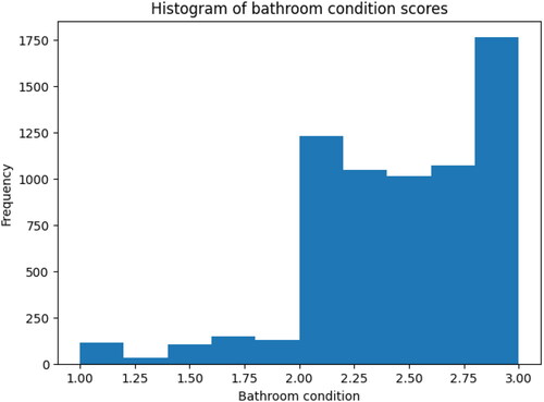
Table 4. Descriptive statistics for numerical attributes in Oslo.

Attribute	Mean	Std	Min	25%	Median	75%	Max
Size	167.4	59.9	51.0	126.0	158.0	199.5	763.0
Build year	1969	29	1745	1955	1971	1986	2018
Building framework	2.549	0.410	1.000	2.200	2.600	3.000	3.000
Plot	2.352	0.517	1.000	2.000	2.333	2.996	3.000
Windows	2.363	0.527	1.000	2.000	2.000	3.000	3.000
Doors	2.565	0.420	1.000	2.102	2.506	3.000	3.000
Roof	2.561	0.457	1.000	2.000	2.500	3.000	3.000
Exterior extensions	2.559	0.528	1.000	2.000	3.000	3.000	3.000
Interior surfaces	2.664	0.384	1.000	2.500	2.750	3.000	3.000
Bathroom	2.457	0.438	1.000	2.167	2.500	2.800	3.000
Kitchen	2.669	0.478	1.000	2.000	3.000	3.000	3.000
HVAC, sanitary	2.481	0.454	1.000	2.000	2.500	3.000	3.000

Condition Attributes Correlation

Figure 3 shows the correlation among condition attributes and selected noncondition attributes, including the target variable.

Figure 3. Heatmap displaying correlation between condition attributes and selected noncondition attributes, including the target variable. A number close to 1, or a dark green color, indicates high positive correlation, and a number close to –1, or a light color, indicates high negative correlation.

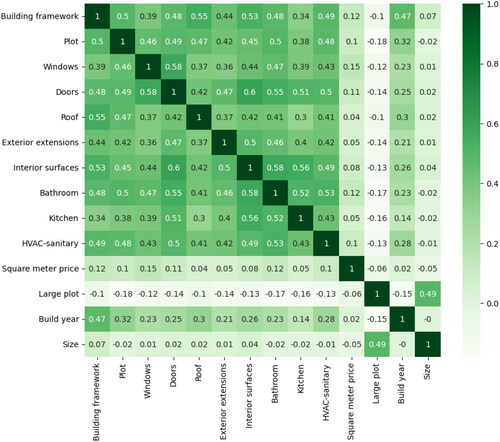
As seen in Figure 3, all condition attributes are positively correlated. This is reasonable, as one should not expect the condition of one attribute to improve as another deteriorates. All condition scores are positively correlated to the square meter price. Additionally, there is no correlation between the size of dwellings and the condition attributes.

Methodology

To assess the explanatory power of dwelling condition in AVMs, three models are used: a hedonic linear regression model, a gradient boosted decision tree known as XGBoost (short for eXtreme Gradient Boosting), and a support vector machine (SVM). This selection provides a variety of distinctly different modeling approaches in terms of both linearity and nonlinearity, as well as the underlying mathematical assumptions.

The models are trained first with and then without condition attributes. The experiment is run first for dwellings in Oslo, then separately for dwellings in Bergen and Trondheim. Bergen and Trondheim are included in the study as a basis of comparison between different urban areas in Norway, which can either increase confidence in the results or uncover discrepancies.

Before running the experiment, the data were randomly split into a training set and a test set. The test set was held out during training and was used only to estimate out-of-sample performance. A 75%/25% split was chosen, based on the recommendation of Hastie et al. (2009).³

To isolate temporal effects in market prices, dummy variables for year and month of sale are included. Moreover, intercept district dummy variables are used to represent the location of dwellings. The district dummy variables are based on statistical districts defined by clustering dwellings on their UTM coordinates using the K-means clustering algorithm (Lloyd, 1982).

Dummy variables are also generated for the building type and district indicators, and any data transformations necessary in the model are performed. All models utilize the logarithm of the square meter price as the target variable, a transformation that is motivated by the distribution seen in Figure 1. The model is then trained using the training set and evaluated using the test set. The root mean square error (RMSE), mean percentage error (MPE), mean absolute percentage error (MAPE), percentage of dwellings within 50% of the actual sale price, and percentage of dwellings within 10% of the actual sale price are noted.

Optimal hyperparameters are found empirically using k-fold cross-validation in conjunction with grid search for XGBoost and random search for the SVM. To analyze the explanatory power of dwelling condition in the machine learning models, a framework known as SHAP is utilized. Following are descriptions of the methods and techniques used in the study. The full mathematical derivations are complex, and the reader is encouraged to refer to the referenced papers for further details.

Hedonic Linear Regression

Hedonic linear regression relies on the hedonic pricing theory outlined by Rosen (1974). The regression equation for dwelling i is given by: (1) $$\hspace{0.17em}\ln \hspace{0.17em}(P_i)={\beta }_0+\sum {\beta }_k{X}_{ki}+{ϵ}_i,\mathrm{\hspace{1em}}\mathrm{\hspace{1em}}\epsilon \Rightarrow \mathrm{i}.\mathrm{i}.\mathrm{d}.$$(1) where k is the number of attributes, X_ki is attribute k for dwelling i, β_k is the regression coefficient for attribute k, β₀ is the bias term, and ϵ_i is the residual. The attributes consist of the ten dwelling conditions, size, a dummy variable for a large plot, dummy variables describing location, dummy variables for housing type, time-related dummies (sales year and sales month), dummy variables for the year of construction, and size-related dummy variables to account for nonlinear relationships.

This study uses least absolute deviation (LAD) robust regression (Koenker & Bassett, 1978) to estimate Equation 1(1) $$\hspace{0.17em}\ln \hspace{0.17em}(P_i)={\beta }_0+\sum {\beta }_k{X}_{ki}+{ϵ}_i,\mathrm{\hspace{1em}}\mathrm{\hspace{1em}}\epsilon \Rightarrow \mathrm{i}.\mathrm{i}.\mathrm{d}.$$(1) based on the findings of Janssen et al. (2001) and Yoo (2001). LAD estimates the optimal regression coefficients in Equation 1(1) $$\hspace{0.17em}\ln \hspace{0.17em}(P_i)={\beta }_0+\sum {\beta }_k{X}_{ki}+{ϵ}_i,\mathrm{\hspace{1em}}\mathrm{\hspace{1em}}\epsilon \Rightarrow \mathrm{i}.\mathrm{i}.\mathrm{d}.$$(1) by solving: (2) $$\arg \underset{{}_{\beta }}{\min }\sum _{i=1}^n|P_i-\beta X_i|$$(2) where β is the coefficient vector, P_i is the true price, and X_i is the vector of characteristics for dwelling i. Dummy variables are introduced to the model where necessary.

Support Vector Machine

The SVM was introduced in 1995 and extended to regression in 1996 (Drucker et al., 1997). This study employs the Scikit-learn implementation for Python (Pedregosa et al., 2011).

The SVM finds a regression line by solving the primal optimization problem given by: (3) $$\underset{{}_{w,b,\zeta ,{\zeta }^{*}}}{\min }\frac{1}{2}{w}^{T}w+C\sum _{i=1}^n({\zeta }_i+{\zeta }_i^{*})$$(3) subject to (4) $$y_i-w^T\varphi (x_i)-b\le ϵ+{\zeta }_i,$$(4) (5) $$w^T\varphi (x_i)+b-y_i\le ϵ+{\zeta }_i^{*}$$(5) (6) $${\zeta }_i,{\zeta }_i^{*}\ge 0,\hspace{1em}i=1,\dots ,n$$(6) where w is a vector of weights, ζ_i and ${\zeta }_i^{*}$ are slack variables, y_i is the target variable, $\varphi (x_i)$ is a mapping of the input vector x to a feature space, b is the bias term, ϵ is the error tolerance threshold, n is the number of training examples, and C is a free parameter controlling the strength of the penalization of erroneous prediction.

The primal problem can be rewritten in its corresponding dual form given by: (7) $$\underset{{}_{\alpha ,{\alpha }^{*}}}{\min }\frac{1}{2}{(\alpha -{\alpha }^{*})}^T(\alpha -{\alpha }^{*})K(x_i,x_j)+ϵ\sum _{i=1}^n({\alpha }_i+{\alpha }_i^{*})+\sum _{i=1}^n{y}_i({\alpha }_i-{\alpha }_i^{*})$$(7) subject to (8) $$\sum _{i=1}^n({\alpha }_i-{\alpha }_i^{*})=0,$$(8) (9) $${\alpha }_i\ge 0,{\alpha }_i^{*}\le C,\hspace{1em}i=1,\dots ,n$$(9) where $K(x_i,x_j)$ is a kernel function and α, ${\alpha }^{*}$ are the vectors of dual coefficients.

After solving the dual problem, the final regression function can be expressed by: (10) $$f(x)=\sum _{i\in SV}({\alpha }_i-{\alpha }_i^{*})K(x_i,x_j)+b$$(10) where b can be calculated according to: (11) $$b=y_i-\sum _{i=1}^n{\alpha }_i^{*}K(x_i,x_j)-ϵ,\hspace{1em}\forall i\text{ such that }0<{\alpha }_i^{*}<C$$(11)

The SVM is sensitive to differences in magnitude of the input data. As a result, the input attributes were scaled to the range of $[0,1],$ as described by Chen et al. (2017).

XGBoost

XGBoost is a highly efficient and optimized implementation of gradient boosted decision trees (Chen & Guestrin, 2016). In this study, the native Python implementation of XGBoost was used.⁴

XGBoost builds an ensemble of regression trees. The predicted output for a given training example ($x_i\in {\mathbb{R}}^m,y_i\in \mathbb{R}$) is the sum of the leaf weights for all trees in the example. This is described mathematically as: (12) $$\widehat{y_i}=\varphi (x_i)=\sum _{k=1}^K{f}_k(x_i),\hspace{1em}{f}_k\in \mathcal{F}$$(12) where $\mathcal{F}=\{f(x)=w_{q(x)}\}$ $(q:{\mathbb{R}}^m\to T,w\in {\mathbb{R}}^T)$ is the space of regression trees. q refers to a specific tree structure that maps an example to one of T leaf nodes. w refers to the weights of the leaf nodes in the tree. Each f_k thus corresponds to the weight of the leaf node that is reached when traversing the independent tree structure q for the given example x.

To build an optimal regressor, XGBoost minimizes the objective function: (13) $$L^{(t)}=\sum _{i=1}^{n}l(y_i,{\widehat{y}}^{(t-1)}+f_{(t)}(x_i))+\Omega (f_t)$$(13) where (14) $$\Omega (f_t)=\gamma T+\frac{1}{2}\lambda \left|\right|w|{|}^2$$(14) where $L^{(t)}$ represents the objective value at the t-th iteration, l is a convex differentiable loss function, y_i is the true output, $y_i^{(t-1)}$ is the prediction of the $(t-1)$-th decision tree, and $f_{(t)}(x_i)$ is the output of the t-th decision tree. $\Omega (f_t)$ is a regularization term in which T is the number of leaves in the tree, γ is a pruning factor, λ is the regularization factor, and w is the output values of the tree.

To reduce mathematical complexity, the loss function is approximated by a second-order Taylor expansion. To minimize, the loss function is differentiated and set equal to zero. The resulting optimal output value of a leaf j is: (15) $$w_j^{*}=-\frac{\sum _{i\in I_j}{g}_i}{\sum _{i\in I_j}{h}_i+\lambda }$$(15) where I_j is the set of training instances in leaf j and g_i and h_i are the first- and second-order gradients of the loss function, respectively.

The measure used to find the optimal splitting feature for a tree is called similarity and is given by the formula: (16) $${\mathcal{L}}_{\text{split}}=\frac{1}{2}\left[\frac{{\left(\sum _{i\in I_L}{g}_i\right)}^2}{\sum _{i\in I_L}{h}_i+\lambda }+\frac{{\left(\sum _{i\in I_R}{g}_i\right)}^2}{\sum _{i\in I_R}{h}_i+\lambda }-\frac{{\left(\sum _{i\in I}{g}_i\right)}^2}{\sum _{i\in I}{h}_i+\lambda }\right]-\gamma$$(16) where L and R represent the left and right node after splitting, respectively.

SHAP

SHAP (SHapley Additive exPlanations) is a game-theoretic approach that can be used to explain the output of any machine learning model. SHAP uses the concept of Shapley values (Shapley, 1953) to calculate the importance of an input feature according to: (17) $${\varphi }_i=\sum _{S\subseteq F\setminus \left\{i\right\}}\frac{\left|S\right|!(|F|-|S|-1)!}{\left|F\right|!}\left[f_{S\cup \left\{i\right\}}(X_{S\cup \left\{i\right\}})-f_S(X_S)\right]$$(17) where ${\varphi }_i$ is the Shapley value of feature i, F is the set of all features, S is any subset of F not containing feature i, $f_{S\cup \left\{i\right\}}(X_{S\cup \left\{i\right\}})$ is the regression prediction using both feature i and the subset S, and $f_S(X_S)$ is the regression prediction using only feature subset S.

This study utilizes the SHAP Python package (Lundberg & Lee, 2017) to calculate feature importance. The package calculates global feature importance according to: (18) $$I_i=\frac{\sum _{j=1}^n\left|{\varphi }_i^j\right|}{n}$$(18) where I_i is the global importance of attribute i, ${\varphi }_i^j$ is the SHAP value of attribute i in training example j, and n is the total number of training examples.

Although SHAP values provide a unified method of explaining any machine learning model, it is important to keep in mind that such explanations only show that a feature provides explanatory power to the model and do not necessarily say anything about causality. Causal effects are complex, and machine learning models are likely to suffer from correlations between included features and unobserved, true causal effects.

Additionally, regularized models, such as XGBoost and the SVM, often rely on as few features as possible to avoid overfitting during training. In the case of correlated features, the model may end up identifying a feature as an important predictor because it summarizes multiple other correlated features. For this reason, SHAP values are used in this paper only to examine explanatory power, not causality.

Results and Discussion

This section presents and discusses the results of the study. The difference in predictive performance with and without condition attributes is analyzed, followed by an analysis of model interpretations. The primary focus is on the results for dwellings in the Oslo data set, and results for Bergen and Trondheim are commented on for robustness.

Model Performance

Table 5 presents the out-of-sample performance results for all models with and without condition attributes in all cities.⁵ All models have a small but observable decrease of similar magnitude in MAPE, ranging from a decrease of 3.39% for XGBoost in Oslo to 6.48% for the linear regression (LR) model in Trondheim. The remaining metrics are also mostly improved by the inclusion of condition attributes, with the exceptions of RMSE for the LR and SVM models, MPE for the XGBoost model, number of dwellings predicted within 50% of actual sale price for the SVM, and number of dwellings predicted within 10% of actual sale price for the LR model in Oslo. This is likely attributable to the fact that the metrics are sensitive to outliers, which are more prominent in the Oslo data set.

Table 5. Test set performance for the linear regression (LR), XGBoost and SVM models with and without condition for dwellings in Oslo, Bergen, and Trondheim.

Model	Location	Condition	RMSE	MPE	MAPE	50%	10%
LR	Oslo	$\square$	9368.90	1.470	12.83	98.44%	50.99%
			9402.84	1.205	12.26	98.50%	52.50%
	Bergen	$\square$	6372.40	1.855	13.83	97.98%	49.06%
			6052.45	1.644	13.19	98.39%	48.39%
	Trondheim	$\square$	6352.88	2.165	13.43	97.86%	48.57%
			6204.51	1.439	12.56	98.57%	54.29%
SVM	Oslo	$\square$	9516.47	1.693	13.18	98.62%	50.45%
			9586.79	1.313	12.59	98.32%	51.59%
	Bergen	$\square$	6487.40	1.590	13.97	97.98%	47.58%
			6136.81	1.329	13.41	98.39%	48.79%
	Trondheim	$\square$	6587.25	1.849	13.85	97.62%	50.48%
			6335.93	1.474	13.04	98.33%	50.71%
XGBoost	Oslo	$\square$	9304.98	2.899	12.99	98.44%	50.81%
			9192.79	3.057	12.55	98.56%	52.14%
	Bergen	$\square$	6368.57	3.454	14.32	97.98%	47.85%
			6078.28	3.444	13.72	98.52%	49.19%
	Trondheim	$\square$	6509.02	3.886	13.71	97.14%	51.19%
			6363.82	3.223	13.04	97.62%	54.05%

Note: The best result for each city is highlighted in bold.

It is evident that all models benefited in terms of predictive accuracy from the inclusion of condition attributes. The small but observable improvement in several metrics in all three regions suggests that dwelling condition contributes additional explanatory power not already present in conventionally considered attributes such as age, location, and size. The results also indicate that linear and nonlinear models may benefit on a similar magnitude in terms of predictive accuracy from the inclusion of condition attributes. The size of the improvement was in line with our expectations.

Model Interpretations

The degree to which dwelling condition provides additional explanatory power can be further explored by examining the coefficients of the linear regression model and the feature importance of the XGBoost and SVM models.

Table 6 shows the regression coefficients for the condition attributes in the linear regression model for dwellings in Oslo, Bergen, and Trondheim. Regression coefficients for all variables in the model are provided in Table C.1. For dwellings in Oslo, six out of the ten condition attributes are deemed statistically significant at 5%, and all significant attributes have positive coefficients. A positive coefficient implies that better condition results in a higher price. In terms of magnitude, the bathroom condition is most important, while the conditions of the doors, roof, HVAC and sanitary equipment, and exterior extensions are all statistically insignificant. For Bergen and Trondheim, four and five out of the ten condition attributes are statistically significant at 5%, respectively. The condition of the bathroom has one of the largest coefficients of the condition attributes in both data sets. Some of the nonsignificant coefficients are negative, but this is not uncommon in a simple linear model with such a high correlation between the dwelling conditions. This is a significant reason why we apply nonlinear models.

Table 6. Linear regression coefficients for condition attributes in Oslo, Bergen, and Trondheim.

	Coefficient
Attribute	Oslo	Bergen	Trondheim
Building framework	0.0322***	0.0117	0.0883***
Plot	0.0198***	0.0147	0.0415***
Windows	0.0134**	0.0069	0.0338***
Doors	0.0067	–0.0002	–0.0146
Roof	–0.0085	0.0172	0.0046
Exterior extensions	0.0007	–0.0077	0.0145
Interior surfaces	0.0338***	0.0441***	–0.0024
Bathroom	0.0382***	0.0337***	0.0565***
Kitchen	0.0203***	0.0186**	0.0063
HVAC, sanitary	0.0030	0.0586***	0.0394***
Dwelling attributes	Yes	Yes	Yes
Time FE	Yes	Yes	Yes
Location FE	Yes	Yes	Yes

Note: The model performance is described in Table 5. Dwelling attributes (size, large plot, dwelling type built year), time FE (sold year, sold month), and location FE (location). The full regression results for Oslo are presented in Appendix C.

*** indicates significance at 1% and ** indicates significance at 5%.

Similar patterns in the importance of condition attributes and their relationship to price were observed in XGBoost and the SVM. Figure 4 shows the importance of features and beeswarm plots for XGBoost in Bergen and Oslo and the SVM in Oslo. The importance of an attribute is determined by its mean absolute SHAP value for all training examples. Greater importance means that the attribute provides more information when making a prediction, and the size of the bar indicates the attribute’s relative importance. In the beeswarm plots, the SHAP value of every condition attribute in each training sample is plotted along the x-axis. The color of the dot indicates the value of the condition attribute in that training sample. In this case, blue dots indicate a worse condition, and red dots indicate a better condition.

Figure 4. XGBoost and SVM model interpretation plots in Oslo. (a) and (c) illustrate the relative importance of the attributes, with larger bars indicating higher importance. (b) and (d) illustrate the identified relationship between price and the condition attributes. The SHAP value represents the estimated impact on the square meter price in NOK. For each attribute, the dots represent a dwelling in the data set. The color of the dot indicates the condition of that attribute, with more blue dots indicating worse condition. Clustering of blue dots to the left and red dots to the right indicates a positive relationship, i.e., a better condition results in a higher price.

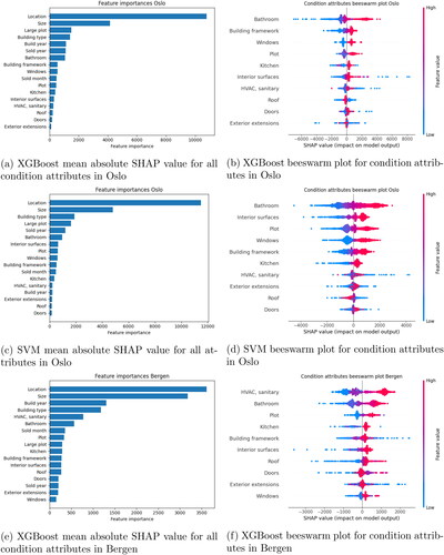
Figure 4(a,c,e) shows, as one would expect, that location and size dominate in terms of importance. The impact of the condition of the bathroom is similar to that of the remaining noncondition attributes, while the impact of the other condition attributes is in the next tier down. Altogether, the 10 dwelling conditions significantly contribute to price prediction in the various models.

Additionally, the impact of the condition of the roof, doors, and exterior extensions is consistently reported to be low. It is worth noting that it may be difficult to interpret SHAP values to assign true importance when there is a high correlation between eatures. This can manifest, for example, as inconsistencies between the values reported for different models. Tree-based models like Boosting, which we have included, are more resilient to correlated features. We also observe significant consistency in the results between the two nonlinear models, further supporting model interpretation.

In the terms of relationship to price, Figure 4(b,d,f) shows that both models indicate a clear relationship in which a better condition of the condition attributes with the greatest importance results in a higher price. This can be seen from the clustering of blue dots to the left and red dots to the right for these attributes. For the less important condition attributes, the dots are more dispersed, and the relationship is less clear. Figure 4(e,f) also illustrates that there are variations in the ranking of feature importances across cities. The full set of model interpretations for Bergen and Trondheim are omitted for brevity, but they follow the same pattern.

For Oslo, we see this relationship quite clearly for bathroom, building framework, windows, plot, and kitchen in both XGBoost and SVM. For interior surfaces, we observe clear clustering in SVM, while in XGBoost, there are some blue points far to the right. One explanation could be that these are renovation projects. For HVAC, sanitary, roof, doors, and exterior extensions, the color relationships are less clear. When combined with the low weight attributed to the conditions of these building elements, they are given little weight and have an unclear influence on price prediction. In Bergen, HVAC and sanitary have high feature importance and show fine clustering. This may indicate that this variable is used differently by appraisers in Bergen compared to those in Oslo. For example, there might be a clearer correlation with the condition of the bathroom in Bergen. Once again, there are clear similarities to the linear models. The results strongly suggest that buyers assign little importance to roof, doors, and exterior extensions when bidding on and buying a home.

There are three important takeaways from the analysis of the model interpretations across the three cities. First, there is consistency between the linear and nonlinear models regarding which condition attributes are ranked high in terms of feature importance and the relationship between these attributes and price. Second, this consistency between models is observed in each region. Third, the identified relationship between condition attributes and price is consistent with the findings of Kain and Quigley (1970), Ooi et al. (2014), and Mathur (2019). These takeaways are further evidence that the performance gain observed when condition attributes are included is not by chance and that dwelling condition provides additional explanatory power to linear and nonlinear AVMs.

It appears that home buyers pay the most attention to the condition of the housing elements that are easy to assess visually when walking around the property. Home buyers seem to consider the technical descriptions in the sales documents to a lesser extent, even though these elements can be just as expensive to deal with, f not more so.

SHAP also allows a deeper analysis of condition attributes and price. Figure 5 shows the relationship between the condition of the bathroom and the building framework, the two condition attributes with the highest feature importance, and the price of dwellings in Oslo, as determined by the XGBoost model. Each dot corresponds to a dwelling in the data set. The dwellings are plotted according to the condition score on the x-axis, and the determined impact that condition score has on the predicted price on the y-axis. The dwellings are also colored according to a second attribute to illustrate interaction effects. In Figure 5(a,c), red dots indicates dwellings with an above-average square meter price and blue dots if below average. In Figure 5(b,d), red dots indicate dwellings located within a given statistically generated cluster and blue dots if not.

Figure 5. Relationship between price and bathroom and building framework condition attributes. Each dot represents a training example. The x-axis holds the value of the condition attribute for that training example, with worse conditions to the left. The y-axis holds the SHAP value, which is the estimated impact on the square meter price in NOK. The dots are colored according to binary variables to illustrate interaction effects.

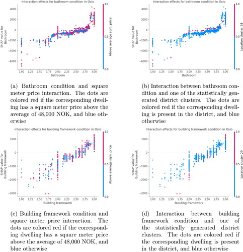
There are some additional insights to be gained from examining the figures. First, they are further evidence that XGBoost has determined a clear relationship in which a better condition results in a higher price for both attributes. This is illustrated by the distinctive upward-sloping shape of the cluster of dots as the condition improves. Second, they illustrate that the relationship is not equal for both attributes. While the relationship between price and condition of the building framework seen in Figure 5(c,d) seems to be fairly linear, the relationship between price and condition of the bathroom is more complex. The trend in Figure 5(a,b) indicates that there is a markedly sharp drop in price when the bathroom condition is slightly degraded from close to 3.0 to 2.75, as can be seen from the sharp dip in the general trend in this range. The price does not seem to be impacted as much in the range of 2.75 to 2.0, where the dots tend to follow a flat, linear shape. Finally, the trend indicates that the price falls at a steeper rate when the condition moves beyond 2.0 toward 1.0, where there is another sharp dip.

Third, the figures allow an examination of interaction effects with other variables. Figure 5(b,d) highlights the interaction effects between the condition attributes and location. The statistically defined cluster with the strongest interaction for the attribute is used as an example. Figure 5(b) indicates that dwellings located in cluster 34 command a higher price for a given bathroom condition in the range of 2.0 to 2.75. This can be seen from the red dots locatedg higher on the y-axis in this range. Similarly, Figure 5(d) indicates that dwellings located in cluster 29 command a lower price for a given building framework condition in the range of 1.5 to 2.75, as can be seen by the red dots located lower on the y-axis in this range. Figure 5(a,c) indicates that the condition’s impact on price is not dependent on the general price level, as can be seen from the dispersion of red dots along the y-axis in both figures.

Last, the greater dispersion of dots for the ratings between 2.0 and 1.0 indicates that the model is less accurate for samples with condition scores in this range. This is hypothesized to be a consequence of the skewed distribution of condition scores toward higher values, making it harder for the model to determine the relationship between higher condition scores and price. Overall, these plots illustrate that the relationship between dwelling condition and price is complex; therefore, further investigation may lead to additional insights.

Conclusion

Real estate is a crucial asset class with significant implications for individuals, institutions, and governments alike. Accurately valuing properties is important for a variety of reasons, from aiding prospective buyers and mortgage lenders to informing tax assessments. The value of a home is influenced by a multitude of characteristics, making it a complex task to determine its true worth. These characteristics include factors such as the home’s location, size, age, and condition, as well as any unique features or amenities it may possess. Properly accounting for these factors is essential for achieving accurate valuations.

In recent years, computer-assisted automated valuations have emerged as a popular and practical tool for valuing properties. These models rely on sophisticated algorithms that consider a range of variables to predict a property’s value. To achieve high levels of accuracy, it is important to identify variables with significant explanatory power. Using machine learning techniques to develop automated valuation models (AVMs) can also provide useful insights into the relationship between variables. Explanatory AI tools such as SHAP can elucidate these connections, enabling a deeper understanding of the factors that drive property values. This information can be valuable for both buyers and sellers, as well as appraisers and researchers seeking to better understand the real estate market.

This study fills a gap in the literature by exploring the explanatory power and price importance of dwelling condition attributes in AVMs. To accomplish this, the study utilizes detailed dwelling condition assessment reports and trains and evaluates three AVM models—a hedonic linear regression model, a gradient-boosted decision tree, and a support vector machine—to predict the sale price of properties in three regions in Norway. These models are widely used in AVM literature and provide different approaches to modeling, in terms of both linearity and nonlinearity, as well as the underlying mathematical assumptions. The study analyzes the performance gains and model interpretations resulting from the inclusion of condition attributes to assess the importance of these attributes for price determination.

The inclusion of dwelling condition attributes led to performance gains across all models and regions on several metrics, with similar magnitude improvements observed across all models. Moreover, there was consistency among all models in terms of the impact of condition attributes on predictions, with better conditions leading to higher prices. This consistency, coupled with the consistent performance gains, supports the conclusion that dwelling condition has explanatory power in AVMs.

Acknowledgment

We are indebted to Vendu AI for providing the data. This research has been funded by the Norwegian Research Council. We would like to thank participants and discussants at The 13th Real Estate Markets and Capital Markets Conference and the research meeting at St. Gallen University for their comments. We also wish to express our gratitude to two anonymous reviewers and our editor for their feedback and valuable contributions.

Disclosure Statement

No potential conflict of interest was reported by the author(s).

Additional information

Funding

This work was supported by Norges Forskningsråd.

Notes

1 For a description of membership requirements in Norwegian, see https://www.osloregionen.no/dokumenter/vedtekter/

2 In the original scale, TG 1 is small or moderate faults, and TG 3 is major faults.

3 Measuring the true predictive power of AVMs is often done with out-of-time predictions. As our primary focus is relative gains, we apply a cross-validation approach.

4 See https://xgboost.readthedocs.io/.

5 The reason why the SVM and XGBoost do not systematically do better than the LR is that we have imposed the same limitation on the SVM and the XGBoost as on the LR. Especially related to time and location, this gives lower explanatory power. We made this choice so that the results were more comparable and thus more interpretable.

Appendix A.

Descriptive Statistics for Numerical Attributes in Bergen and Trondheim

Table A1. Descriptive statistics for numerical attributes in Bergen.

Attribute	Mean	Std	Min	25%	Median	75%	Max
Size	146.3	55.60	51.00	110.0	139.0	177.0	520.0
Build year	1967	37	1685	1954	1971	1993	2017
Building framework	2.642	0.371	1.000	2.375	2.750	3.000	3.000
Plot	2.337	0.514	1.000	2.000	2.000	3.000	3.000
Windows	2.437	0.539	1.000	2.000	2.500	3.000	3.000
Doors	2.703	0.387	1.000	2.500	3.000	3.000	3.000
Roof	2.540	0.446	1.000	2.000	2.500	3.000	3.000
Exterior extensions	2.609	0.491	1.000	2.000	3.000	3.000	3.000
Interior surfaces	2.707	0.366	1.000	2.500	2.769	3.000	3.000
Bathroom	2.361	0.473	1.000	2.000	2.333	2.778	3.000
Kitchen	2.726	0.458	1.000	2.500	3.000	3.000	3.000
HVAC, sanitary	2.495	0.415	1.000	2.000	2.500	3.000	3.000

Table A2. Descriptive statistics for numerical attributes in Trondheim.

Attribute	Mean	Std	Min	25%	Median	75%	Max
Size	162.3	54.59	52.00	124.0	151.0	190.0	444.0
Build year	1973	24	1842	1961	1973	1988	2018
Building framework	2.702	0.339	1.250	2.400	2.800	3.000	3.000
Plot	2.606	0.373	1.000	2.333	2.667	3.000	3.000
Windows	2.530	0.481	1.000	2.000	2.712	3.000	3.000
Doors	2.690	0.412	1.000	2.500	3.000	3.000	3.000
Roof	2.707	0.395	1.000	2.500	3.000	3.000	3.000
Exterior extensions	2.705	0.445	1.000	2.407	3.000	3.000	3.000
Interior surfaces	2.708	0.430	1.000	2.333	3.000	3.000	3.000
Bathroom	2.454	0.409	1.000	2.000	2.500	2.750	3.000
Kitchen	2.780	0.385	1.000	2.667	3.000	3.000	3.000
HVAC, sanitary	2.664	0.425	1.000	2.331	3.000	3.000	3.000

Appendix B.

Maps of Areas Used in the Study

Figure B1. Oslo and Viken county, with the main area of study highlighted. The city of Oslo is marked in black. The numbering of the municipalities is as follows: 1. Oslo, 2. Lørenskog, 3. Bærum, 4. Lillestrøm, 5. Asker, 6. Drammen.

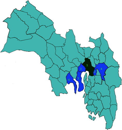
Figure B2. Map of boroughs in Oslo, color-coded according to average dwelling square meter price. Square meter prices are retrieved from Oslo municipality fact database (Oslo Municipality, 2021). No price information was provided for the center of Oslo, colored in blue. Red color indicates higher prices, green color indicates lower prices. The prices range from around NOK 43,000 to NOK 90,000.

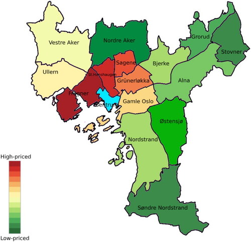
Figure B3. Map of boroughs in Trondheim, color-coded according to average dwelling square meter price. Prices range from around NOK 34,000 to NOK 51,000 and are for the last quarter of 2020. Prices are retrieved from Krogsveen (2021).

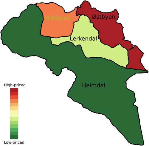
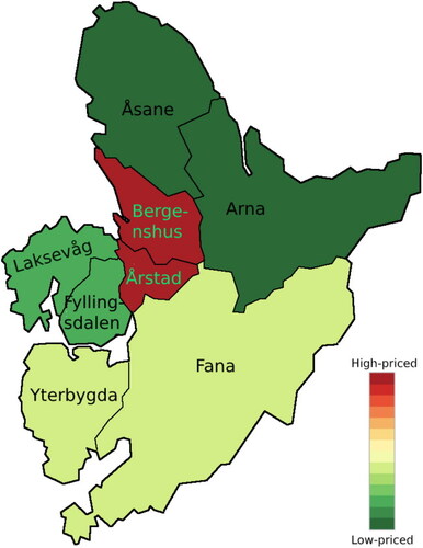
Figure B4. Map of boroughs in Bergen, color-coded according to average dwelling square meter price. Prices range from around NOK 30,000 to NOK 50,000 and are for 2020. Prices are retrieved from Marschhäuser (2021).

Appendix C.

Regression Results

Table C1. Full regression results for Oslo.

	Coef	Std err	$\mathbf{P}>\left|\mathbf{z}\right|$
Const	10.6523	0.038	0.000
Building fwk.	0.0322	0.008	0.000
Plot	0.0198	0.006	0.000
Windows	0.0134	0.005	0.014
Doors	0.0067	0.008	0.375
Roof	– 0.0085	0.006	0.154
Exterior ext.	0.0007	0.005	0.883
Interior surf.	0.0338	0.008	0.000
Bathroom	0.0382	0.007	0.000
Kitchen	0.0203	0.006	0.001
HVAC	0.0030	0.006	0.628
Size	– 0.0017	0.000	0.000
Large plot	0.0755	0.006	0.000
Location 0	–0.2045	0.019	0.000
Location 10	0.2108	0.021	0.000
Location 11	0.4482	0.019	0.000
Location 12	–0.1235	0.023	0.000
Location 13	–0.4448	0.018	0.000
Location 14	0.1430	0.019	0.000
Location 15	–0.1195	0.019	0.000
Location 16	0.2151	0.020	0.000
Location 17	0.1128	0.019	0.000
Location 18	–0.2310	0.023	0.000
Location 19	0.2947	0.019	0.000
Location 2	–0.4052	0.018	0.000
Location 20	–0.2643	0.019	0.000
Location 21	–0.0948	0.025	0.000
Location 22	0.0132	0.020	0.504
Location 23	–0.4757	0.019	0.000
	Coef	Std err	[0.025
Location 24	–0.0922	0.024	0.000
Location 25	–0.0774	0.021	0.000
Location 26	0.5689	0.030	0.000
Location 27	–0.2398	0.022	0.000
Location 28	0.3271	0.021	0.000
Location 29	0.4572	0.020	0.000
Location 3	0.2460	0.021	0.000
Location 30	0.2106	0.019	0.000
Location 31	0.0509	0.020	0.012
Location 32	0.3408	0.020	0.000
Location 33	–0.0961	0.021	0.000
Location 34	0.4700	0.018	0.000
Location 35	–0.2471	0.021	0.000
Location 36	–0.3310	0.034	0.000
Location 37	0.2976	0.019	0.000
Location 38	0.0022	0.023	0.925
Location 39	–0.1175	0.022	0.000
Location 4	0.2967	0.019	0.000
Location 5	0.3196	0.020	0.000
Location 6	–0.0509	0.020	0.010
Location 7	–0.0306	0.019	0.110
Location 8	–0.5271	0.020	0.000
Location 9	–0.2330	0.021	0.000
Apartment block	–0.0357	0.027	0.181
Detached house	0.1082	0.007	0.000
Semidetached house	0.0408	0.007	0.000
Sold year 2017	0.0778	0.009	0.000
Sold year 2018	0.0814	0.008	0.000
Sold year 2019	0.1304	0.009	0.000
	Coef	Std err	$\mathbf{P}>\left|\mathbf{z}\right|$
Sold year 2020	0.1041	0.032	0.001
Sold month 10	0.0267	0.011	0.015
Sold month 11	0.0286	0.011	0.009
Sold month 12	0.0358	0.011	0.001
Sold month 2	–0.0182	0.011	0.109
Sold month 3	0.0083	0.012	0.484
Sold month 4	–0.0067	0.012	0.563
Sold month 5	0.0119	0.012	0.308
Sold month 6	0.0295	0.011	0.005
Sold month 7	0.0247	0.010	0.018
Sold month 8	0.0281	0.010	0.007
Sold month 9	0.0326	0.011	0.003
Built 1950–1970	–0.1449	0.011	0.000
Built 1970–1990	–0.1299	0.011	0.000
Built 1990–2000	–0.0964	0.013	0.000
Built 2000–2010	–0.0416	0.012	0.001
Built <1950	–0.0983	0.012	0.000
Size 110–130	–0.1191	0.022	0.000
Size 130–150	–0.1480	0.025	0.000
Size 150–170	–0.1663	0.028	0.000
Size 170–190	–0.1849	0.031	0.000
Size 190–210	–0.1966	0.035	0.000
Size 210–250	–0.2103	0.040	0.000
Size 250–300	–0.2276	0.049	0.000
Size 300–350	–0.1588	0.061	0.009
Size 350–400	–0.0338	0.074	0.649
Size 70–90	–0.0300	0.021	0.150
Size 90–110	–0.0872	0.020	0.000
Size >400	0.2524	0.102	0.013

References

- Anderson, J. T., Fuerst, F., Peiser, R. B., & Seiler, M. J. (2023). iBuyer’s use of proptech to make large-scale cash offers. Journal of Real Estate Research. Advance online publication. https://doi.org/10.1080/08965803.2023.2214467
- Antipov, E., & Pokryshevskaya, E. (2012). Mass appraisal of residential apartments: An application of random forest for valuation and a CART-based approach for model diagnostics. Expert Systems with Applications, 39, 1772–1778. https://doi.org/10.1016/j.eswa.2011.08.077
- Bergen Municipality. (2020). Fakta om Bergen [Facts about Bergen]. https://www.bergen.kommune.no/omkommunen/fakta-om-bergen/befolkning/befolkning
- Chen, J.-H., et al. (2017). Forecasting spatial dynamics of the housing market using support vector machine. International Journal of Strategic Property Management, 21, 273–283. https://doi.org/10.3846/1648715X.2016.1259190
- Chen, T., & Guestrin, C. (2016). Xgboost: A scalable tree boosting system. In Proceedings of the 22nd ACM Sigkdd International Conference on Knowledge Discovery and Data Mining (pp. 785–794). Association for Computing Machinery.
- Cortes, C., & Vapnik, V. (1995). Support-vector networks. Machine Learning, 20, 273–297. https://doi.org/10.1023/A:1022627411411
- Dimopoulos, T., Tyralis, H., Bakas, N. P., & Hadjimitsis, D. (2018). Accuracy measurement of random forests and linear regression for mass appraisal models that estimate the prices of residential apartments in Nicosia, Cyprus. Advances in Geosciences, 45, 377–382. https://doi.org/10.5194/adgeo-45-377-2018
- Do, A. Q., & Grudnitski, G. (1992). A neural network approach to residential property appraisal. The Real Estate Appraiser, 58, 38–45.
- Doumpos, M., Papastamos, D., Andritsos, D., & Zopounidis, C. (2021). Developing automated valuation models for estimating property values: A comparison of global and locally weighted approaches. Annals of Operations Research, 306, 415–433. https://doi.org/10.1007/s10479-020-03556-1
- Drucker, H., Burges, C. J., Kaufman, L., Smola, A., & Vapnik, V. (1996). Support vector regression machines. In M. C. Mozer, M. I. Jordan, & T. Petsche (Eds.), Advances in neural information processing systems 9 (pp. 155–161). MIT Press.
- Graczyk, M., Lasota, T., Trawiński, B., & Trawiński, K. (2010). Comparison of bagging, boosting and stacking ensembles applied to real estate appraisal. In M. T. Le, J. Swiatek, N. T. Nguyen (Eds.), Intelligent information and database systems: Second International Conference, ACIIDS, Hue City, Vietnam, March 24-26, 2010, proceedings, part II 2 (pp. 340–350). Springer Berlin Heidelberg. https://doi.org/10.1007/978-3-642-12101-2_35
- Harrison, D. M., Seiler, M. J., & Yang, L. (2023). The impact of iBuyers on housing market dynamics. The Journal of Real Estate Finance and Economics. Advance online publication. https://doi.org/10.1007/s11146-023-09954-zAU
- Hastie, T., Tibshirani, R., & Friedman, J. (2009). The elements of statistical learning: Data mining, inference, and prediction (p. 222). Springer.
- Helbich, M., & Griffith, D. A. (2016). Spatially varying coefficient models in real estate: Eigenvector spatial filtering and alternative approaches. Computers, Environment and Urban Systems, 57, 1–11. https://doi.org/10.1016/j.compenvurbsys.2015.12.002AU
- Helgaker, E., Oust, A., & Pollestad, A. J. (2023). Adverse selection in iBuyer business models—don’t buy lemons! Zeitschrift für Immobilienökonomie, 9(2), 109–138. https://doi.org/10.1365/s41056-022-00065-z
- Ho, W. K. O., Tang, B.-S., & Wong, S. W. (2021). Predicting property prices with machine learning algorithms. Journal of Property Research, 38(1), 48–70. https://doi.org/10.1080/09599916.2020.1832558
- Janssen, C., Söderberg, B., & Zhou, J. (2001). Robust estimation of hedonic models of price and income for investment property. Journal of Property Investment & Finance, 19, 342–360. https://doi.org/10.1108/EUM0000000005789
- Kain, J. F., & Quigley, J. M. (1970). Measuring the value of housing quality. Journal of the American Statistical Association, 65, 532–548. https://doi.org/10.1080/01621459.1970.10481102
- Koenker, R., & Bassett, G., Jr. (1978). Regression quantiles. Econometrica, 46(1), 33–50. https://doi.org/10.2307/1913643
- Kok, N., Koponen, E.-L., & Martínez-Barbosa, C. A. (2017). Big data in real estate? From manual appraisal to automated valuation. The Journal of Portfolio Management, 43, 202–211. https://doi.org/10.3905/jpm.2017.43.6.202
- Kontrimas, V., & Verikas, A. (2011). The mass appraisal of the real estate by computational intelligence. Applied Soft Computing, 11, 443–448. https://doi.org/10.1016/j.asoc.2009.12.003
- Krogsveen. (2021). Prisutvikling for Norge. https://www.krogsveen.no/prisstatistikk?
- Lam, K. C., Yu, C. Y., & Lam, C. K. (2009). Support vector machine and entropy based decision support system for property valuation. Journal of Property Research, 26(3), 213–233. https://doi.org/10.1080/09599911003669674
- Lin, C., & Mohan, S. (2011). Effectiveness comparison of the residential property mass appraisal methodologies in the USA. International Journal of Housing Markets and Analysis, 4, 224–243. https://doi.org/10.1108/17538271111153013
- Lloyd, S. (1982). Least squares quantization in PCM. IEEE Transactions on Information Theory, 28(2), 129–137. https://doi.org/10.1109/TIT.1982.1056489
- Lundberg, S. M. & Lee, S-I. (2017). A unified approach to interpreting model predictions. In I. Guyon, U. Von Luxburg, S. Bengio, H. Wallach, R. Fergus, S. Vishwanathan, and R. Garnett (Eds.), Advances in neural information processing systems 30 (pp. 4765–4774). Curran Associates.
- Mæhlum, L. (2020). Viken i Store norske leksikon [Viken in the great Norwegian encyclopedia]. https://snl.no/Viken
- Marjan, Č., et al. (2018). Estimating the performance of random forest versus multiple regression for predicting prices of the apartments. ISPRS International Journal of Geo-Information, 7, 168. https://doi.org/10.3390/ijgi7050168
- Marschhäuser, S. H. (2021). Ferske boligpriser: Sterk vekst [Recent housing prices: Strong growth]. https://www.bt.no/bolig/i/6zBEmO/ferske-boligpriser-sterk-vekst
- Mathur, S. (2019). House price impacts of construction quality and level of maintenance on a regional housing market: Evidence from King County, Washington. Housing and Society, 46(2), 57–80. https://doi.org/10.1080/08882746.2019.1601928
- Mayer, M., Bourassa, S. C., Hoesli, M., & Scognamiglio, D. (2019). Estimation and updating methods for hedonic valuation. Journal of European Real Estate Research, 12(1), 134–150. https://doi.org/10.1108/JERER-08-2018-0035
- Mimis, A., Rovolis, A., & Stamou, M. (2013). Property valuation with artificial neural network: The case of Athens. Journal of Property Research, 30(2), 128–143. https://doi.org/10.1080/09599916.2012.755558
- Nghiep, N., & Al, C. (2001). Predicting housing value: A comparison of multiple regression analysis and artificial neural networks. Journal of Real Estate Research, 22(3), 313–336. https://doi.org/10.1080/10835547.2001.12091068
- Olaussen, J., Oust, A., & Solstad, J. T. (2017, December). Energy performance certificates: Informing the informed or the indifferent? Energy Policy, 111, 246–254. https://doi.org/10.1016/j.enpol.2017.09.029
- Ooi, J., Le, T. T., & Lee, N.-J. (2014). The impact of construction quality on house prices. Journal of Housing Economics, 26, 126–138. https://doi.org/10.1016/j.jhe.2014.10.001
- Oslo Municipality. (2021). Boligpriser. https://bydelsfakta.oslo.kommune.no/bydel/alle/boligpriser
- Oust, A., Hansen, S. N., & Pettrem, T. R. (2020). Combining property price predictions from repeat sales and spatially enhanced hedonic regressions. The Journal of Real Estate Finance and Economics, 61, 183–207.
- Pedregosa, F., et al. (2011). Scikit-learn: Machine learning in Python. Journal of Machine Learning Research, 12, 2825–2830.
- Renigier-Biłozor, M., Janowski, A., & d’Amato, M. (2019). Automated valuation model based on fuzzy and rough set theory for real estate market with insufficient source data. Land Use Policy, 87, 104021. https://doi.org/10.1016/j.landusepol.2019.104021
- Rosen, S. (1974). Hedonic prices and implicit markets: Product differentiation in pure competition. Journal of Political Economy, 82(1), 34–55. https://doi.org/10.1086/260169
- Seiler, M. J., & Yang, L. (2023). The burgeoning role of iBuyers in the housing market. Real Estate Economics, 51(3), 721–753. https://doi.org/10.1080/08965803.2023.2214467
- Shapley, L. S. (1953). A value for n-person games. Contributions to the Theory of Games, 2(28), 307–317.
- SSB. (2021). Prisstigning for brukte boliger siste ti år [Price increase for used homes in the last ten years]. https://www.ssb.no/bygg-bolig-og-eiendom/faktaside/bolig
- Standard (2012). Bedre tilstandsanalyser med ny NS 3424 [Improved condition analyses with the new NS 3424]. https://www.standard.no/nyheter/nyhetsarkiv/bygg-anlegg-og-eiendom/2012/bedre-tilstandsanalyser-med-ny-ns-3424/
- Standard (2015). Tilstandsanalyse av bolig - NS 3600 [Condition analysis of housing - NS 3600]. https://www.standard.no/fagomrader/bygg-anlegg-og-eiendom/teknisk-tilstandsanalyse-av-bolig---ns-3600/ (visited on 6th June 2021).
- Trondheim Municipality. (2020). Trondheim i tall [Trondheim in numbers]. https://www.trondheim.kommune.no/statistikk/
- Yoo, S.-H. (2001, January). A robust estimation of hedonic price models: Least absolute deviations estimation. Applied Economics Letters, 8, 55–58. https://doi.org/10.1080/135048501750041303