Does Personal Financial Distress Affect Workers’ Performance? Evidence From Real Estate Agents

Abstract

This study examines how personal financial distress affects workers’ performance. Using the real estate brokerage industry as a setting and personal bankruptcy filing as a proxy for personal financial distress, we find that sale prices of agent-represented houses are lower in the year when agents are financially distressed than the non-distressed year, relative to the control group. We also find that the less desirable sales’ outcomes induced by distressed agents spill over to homeowners’ future buying activities. These owners subsequently buy houses with higher loan-to-value (LTV) ratios in lower-quality neighborhoods.

Keywords:

• Personal financial distress
• real estate agents
• spillover effects
• workplace performance

JEL CLASSIFICATION:

• J01
• D10
• L85
• R30

1. Introduction

Intermediaries play a major role in our society, in fact, many firms do not sell products or services directly to consumers, but instead use marketing intermediaries to execute an assortment of necessary functions to get the product to the final user. These intermediaries typically enter into longer-term commitments with the producer and compose what is known as the marketing channel. If intermediaries experience financial distress, it may affect the services provided to the buyer and seller. A good example is how financial intermediaries (i.e., banks) experienced severe financial distress in 2008, which caused a systemic financial crisis and affected the world’s economy. We extend this research topic by examining how personal financial distress affects agents’ services in a residential real estate context.

For several reasons, the real estate brokerage industry provides an excellent setting for testing how personal financial distress affects worker’ performance. First, unlike other working environments where employers set work schedules and employees do not have choices over their labor supply, real estate agents can set their own hours. Because that choice is discretionary for real estate agents, they could easily adjust their listing and selling strategy when facing personal financial events, in contrast with other industries where working hours are fixed. Second, the agency problem is more pronounced in the relationship between real estate agents and their clients¹ compared with other settings, such as the relationship between innovation workers and firms (Bernstein et al., 2021) or between teachers and students (Maturana & Nickerson, 2020). Most industries use a financial incentive to reduce the misalignment of incentives between principals and agents, but the financial incentive structure—that is, the commission structure—fails to mitigate the agency problem in the real estate market. The commission fee features a consistent rate (typically 5–6% of the sale price) across all regions of the country and over time. This percentage-based commission structure provides the agent only a small marginal benefit to exert extra effort (Levitt & Dubner, 2014; Yavas, 2007). For example, a $10,000 decrease in sale price only results in a $300 loss in commission, but saves the agent much effort. Therefore, the real estate market provides a great setting for studies on agency problems. Third, we can observe agents’ performance repeatedly for the same real estate agent over time, which enables us to exploit variations within a real estate agent over time. Fourth, we can track home sellers over time after their first sale and measure changes in leverage and neighborhood when these home sellers subsequently purchase a second house. So, we can directly test the spillover effect from the impact of real estate agents’ financial distress on themselves to the impact on their represented home sellers. Most home sellers use the proceeds from the sale of their previous house to pay for their next home purchase. If real estate agents cause losses for home sellers because of the agents’ financial distress, home sellers may have to distort their subsequent purchase decision. For example, home sellers may have to increase financial leverage or move to worse neighborhoods due to the loss of sale price from their previous house. Therefore, we can take a further step and compare the differences in home purchase decisions, such as the leverage decision and location decision, among home sellers whose houses are represented by distressed agents versus non-distressed ones.

We use personal bankruptcy filing to proxy for an individual’s financial distress, following Maturana and Nickerson (2020) as our main analysis because filing for bankruptcy represents a severe personal financial distress for individuals and a wealth loss large enough to have a real impact on debtors. In a robustness test, we also use local negative housing-related wealth shocks as another proxy for personal financial distress following Bernstein et al. (2021) to further establish the causal relation. We have several challenges to find the effect of personal financial distress on real estate agents’ performance. The first concern is that unobserved agent-level characteristics may drive our results. For example, different agents have different utility functions or different risk preferences. Agents who experienced personal distress may endogenously have a lower performance. We overcome this question by conducting within-agents analysis so that we can fix the agents’ time-invariant characteristics. The second concern is that the local economy may both cause agents to be financially distressed and affect their sale outcomes. To overcome this challenge, we include agents’ location (ZIP code) by year fixed effects. Therefore, all our tests include real estate agent fixed effects to ensure all the analyses are conducted within individuals, and agents’ location by year fixed effects to rule out the possibility that time-varying agents’ local factors drive our results. We also add housing characteristics as well as housing market (county) by year fixed effects as controls. We mainly focus on how personal financial distress affects the selling price of the agent-represented houses since selling price is a real outcome for home sellers. And if personal financial distress has a negative effect on the selling price of client’s house, this negative effect could directly spill over to home sellers and cause home sellers to suffer a loss. Our baseline result shows that the selling price of agent-represented houses is reduced by 4% in the year when real estate agents are financially distressed. Relative to the mean, sale price of clients’ houses drops by $8,938. Moreover, our result confirms that before and after the event, the effect on the selling price is not significant. Instead, the significant and negative effect only takes place in the immediacy of the bankruptcy filing.

Much research in behavioral economics (Carvalho et al., 2016; Di Falco et al. 2019; Tanaka et al., 2010) highlights that a negative income event impacts time discounting and makes people behave more impatiently. Based on these extant literature, we hypothesize that personal financial distress makes real estate agents less patient for monetary reward, which leads to a decrease in time spent on housing search related tasks. This hypothesis is supported by a 3.6% drop in listing price and a 14.1% drop in time-on-market (TOM) of the agent-represented houses in the year when real estate agents are financially distressed. Relative to the mean, the listing price of clients’ houses drops by $8,355, and clients’ houses are sold about 14 days earlier when represented by financially distressed agents. To summarize, agents sell clients’ houses for $8,938 less, but close the deal two weeks earlier in distressed years compared with non-distressed years, relative to agents who have never experienced financial distress.

We also conduct a battery of robustness checks to rule out other possible explanations and ensure our results are not driven by confounding factors. For example, there may be concern of reverse causality, wherein real estate agents’ bankruptcy filings may be endogenously determined by the decline in housing prices. To test this explanation, we restrict the sample to agents whose represented houses are located in areas with increasing home price index (HPI) prior to filing for bankruptcy. Second, we exclude properties located in the same ZIP codes or same counties where real estate agents live to further test if our results are driven by unobserved granular local confounding factors. Next, to rule out the possibility that unobserved house characteristics may drive the result, we use a repeat sale methodology by adding property fixed effects. In addition, to rule out the possibility that unobserved seller characteristics may drive the results, we choose samples with sellers who sell two or more properties and control for seller fixed effects. Also, different firms may have different preferences in the listing and selling decisions, so to overcome this problem, we add firm fixed effects where the listing agents are working as a control. Finally, we also explore another source of personal financial distress, which is the decline of personal real estate wealth. We use variations in the severity of the financial crisis in 2008 and afterwards to create exogenous changes (decline) in agents’ real estate wealth to proxy for personal financial distress to further establish a causal relation between personal financial distress and agents’ performance.

We implement several heterogeneity tests to find where personal financial distress has a more pronounced effect on the selling price of clients’ houses. For example, agents who have a larger personal financial distress may be more affected. We use three indicators to measure the severity of personal financial distress: current income, total debt, and debt-to-income ratio. We find a more pronounced negative effect exists in financially distressed real estate agents with lower income, higher debt, and a higher debt-to-income ratio. We also find the effect is heterogeneous across different real estate market characteristics.

Lastly, we track the home sellers’ future purchases and compare the decision made by home sellers represented by financially distressed brokers versus those represented by non-distressed brokers. Since most home sellers use the proceeds from their previous house to pay for their next house, the loss caused by distressed agents may distort home sellers’ next house purchase decision. We find home sellers whose sold house is represented by financially distressed agents tend to take loans and use higher leverage when they purchase their next house. They are more likely to move to a worse neighborhood with lower household income, education level and housing price. All the above results indicate the negative spillover of personal financial distress from real estate agents to home sellers.

The paper proceeds as follows. Section 2 reviews the literature and develops our hypothesis. Section 3 provides institutional background as well as the data used in this paper. Section 4 discusses the research design and main results. Section 5 shows the spillover effect, while section 6 concludes.

2. Contributions to the Literature

In this section, we review three bodies of literature: the consequences of personal financial distress, the conflict of interest between agents and clients, and the spillover effect and the externality effect of peers. We discuss the potential contributions of our paper to the existing literature and develop our main hypothesis regarding the effect of personal financial distress on real estate agents’ performance based on extant literature.

2.1. Consequences of Personal Financial Distress

The first strand of literature focuses on the real effect of personal financial distress. Personal financial distress has a negative impact on individuals’ consumption. For example, Mian et al. (2015) investigate the consequences of deterioration in household balance sheets and find that the decline in housing wealth leads to a decrease in consumption. Maggio et al. (2019) also provide direct evidence on how debt relief benefits individuals and find that student loan debt relief increases borrowers’ consumption. Personal financial distress also affects individuals’ behaviors. For example, Pool et al. (2019) show that negative housing wealth shocks cause fund managers to reduce risk due to career concerns. Adopting a similar identification strategy, Bernstein et al. (2021) find negative housing wealth shocks to inventors translate into fewer patents and more patents with lower quality. Dimmock et al. (2021) find that advisors increase misconduct following declines in their homes’ values. Cespedes et al. (2020) study how negative housing wealth shocks affect actors’ career choice and find that losses in housing wealth makes homeowners less likely to choose films with high reward. Using a field study and focusing on financially constrained workers, Kaur et al. (2021) find that those who received cash increase performance by 5.3%. Maturana and Nickerson (2020) document that students’ passing rate decreases following a declaration of bankruptcy by their teachers.

We complement this strand of literature in household finance by studying the role that real estate agents play in the housing sale process and how real estate agents’ financial distress affects their performance and further impacts their clients.

2.2. Conflict of Interest between Agents and Clients

The second strand of literature focuses on the conflict of interest between agents and clients—the agency problem. The principal–agent problem is one of the oldest research topics in corporate finance (Geltner et al., 1991; Weisbach, 1988). As an example of the principle-agent problem, the conflict of interest between real estate agents and clients in the real estate market has attracted increased attention from researchers in recent years. Some studies discuss the incentive problem between agents and clients. Rutherford et al. (2005) find that agent-owned houses sell at a higher price, but see no time-on-market difference. They attribute these results to agents’ efforts. Similarly, Levitt and Syverson (2008) find that agent-owned houses sell at a higher price and stay on the market longer, and argue this is due to the agents’ information advantage. Agarwal et al. (2019) argue that agents bought their own houses at prices that are 2.54% lower than comparable houses bought by other buyers. Some studies examine conflict of interest by focusing on steering in the real estate market such as steering consumers to affiliated financial services (Lopez et al., 2022), to affiliated brokerages (i.e., in-house transactions) (Han & Hong, 2016), and to high-commission properties (Barwick et al., 2017; Levitt et al., 2008; Rutherford & Yavas, 2012). In the mortgage market, loan product steering is also documented in the literature. For example, Agarwal et al. (2016) find that lenders steer borrowers to originate mortgage products with high interest rates. Guiso et al. (2022) also confirm the banks’ steering effect, and argue this effect varies based on household sophistication. Agarwal et al. (2020) find that lenders steer borrowers into piggyback loans rather than letting borrowers purchase private mortgage insurance for loans with loan-to-value ratios (LTV) greater than 80%. Some studies focus on market entry as well as competition in the brokerage market. Three works (Barwick & Pathak, 2015; Han & Hong, 2011; Hsieh & Moretti, 2003) on the consequence of free entry of agents in the real estate market find that it led to cost inefficiency and welfare reduction. A cut in commission fee would result in fewer agents, but more welfare for home buyers/sellers. Barwick and Wong (2019) further provide insight for why the commission fee does not change despite the increase in competition and why the failure of competition exists in the real estate agent market. Results are quite opposite in the mortgage market. For example, Robles-Garcia (2019) shows that competition among mortgage brokers facilitates the entry of new lenders, and her structure model estimate finds a ban on commissions leads to a 25% decrease in consumer welfare.

We complement extant literature by analyzing principle-agent problems under agents’ financial distress settings and studying if agents’ financial distress exacerbates principle-agent problems.

2.3. Spillover Effect and Externality Effect of Peers

The third strand of literature focuses on the spillover effect and externality effect of peers. A good example is that there is a series of literature which focuses on the spillover effect of foreclosed properties. For example, Campbell et al. (2011) document that forced sales have spillover effects on the prices of local unforced sales. In particular, they that find that each foreclosure that takes place 0.05 miles away lowers the price of a house by about 1%. Harding et al. (2009) and Gerardi et al. (2015) document that one nearby foreclosed property leads to a 1% selling price discount of a non-distressed property transaction. Anenberg and Kung (2014) try to disentangle two sources, competition and disamenities, and find that the competitive pressure that a foreclosed property exerts on nearby sellers is an important source of the spillover effect. The spillover effect through networks is also a well-known strand of literature. For example, some literature studies how negative events are transmitted through bank-firm networks (Khwaja & Mian, 2008), IT-non-IT firms (Townsend, 2015), internal firm networks (Giroud & Mueller, 2019), and supply chain networks (Barrot & Sauvagnat, 2016). These studies on spillover effects help direct governments to make corresponding bailout policies. For example, due to the negative spillover effects of foreclosure, the U.S. government-initiated programs during the financial crisis to avoid foreclosure and help “underwater houses.” The Home Affordable Refinance Program (HARP) and the Home Affordable Modification Program (HAMP) are two of the most important policies introduced by the U.S. government during the financial crisis. Agarwal et al. (2017, 2023) evaluate those two policies and find there is an increase in consumer spending following their enactment. Moulton et al. (2022) find that there is an increase in wages as well as employment after the receipt of mortgage payment subsides, another federal foreclosure program.

We complement the previous research by analyzing the spillover effect from agents to clients, that is, home sellers. We ask if personal financial distress indeed affects agents’ performance and how it spills over to home sellers through the client-agent connection.

2.4. Hypothesis

Based on prior literature, we examine two competing hypotheses. First, personal financial distress may boost the performance of real estate agents. They may want to work harder to get out of personal financial distress and make up for lost wealth, so they would sell clients’ houses at a higher price for each sale or sell more houses to make more commissions based on the reference income and loss aversion theory documented in the literature (Goette et al., 2004; Rizzo & Zeckhauser, 2003).

Second, behavioral economics research argues that negative income events impact time discounting and make people behave more impatiently when making financial decisions. For example, Tanaka et al. (2010) find evidence suggesting that income has a causal effect on an experimentally measured discount rate in Vietnam. Di Falco et al. (2019) show that severe droughts in Ethiopia led to increases in farmers’ discount rate. Focusing on low-income households in the U.S., Carvalho et al. (2016) show that before a payday, participants are found to be more present biased in intertemporal choices about monetary rewards. So, based on previous literature, we hypothesize that personal financial distress makes real estate agents less patient for monetary reward, which leads to a decrease in time spent on housing-search-related tasks, further leading to a lower selling price. Based on these two competing hypotheses, the effect of personal financial distress is an empirical question.

3. Institutional Background and Data

3.1. Real Estate Agents in U.S

Real estate agents play a major role in residential real estate transactions, wherein the asset is illiquid, lumpy, heterogenous, and traded in decentralized markets, unlike stock markets. Home selling is a time-consuming process, which includes determining the listing price, advertising the homes, matching preferences, and showing homes as well as negotiating prices. Similar issues for the home buying process include visiting houses, negotiating offers, obtaining a mortgage, and closing the deal. Therefore, most home sellers and home buyers hire an agent to facilitate the buying and selling process. According to the 2019 National Association of Realtors Profile of Home Buyers and Sellers,² 89% of all buyers/sellers purchased/sold their home through an agent, an increase of 20 percentage points compared with 69% in 2001, which indicates that real estate agents still play a great role in the Internet era. Real estate agents have access to the Multiple Listing Service (MLS) database and, therefore, can easily improve this matching process. For example, working as a listing agent, the agent advises how much the home seller should list the house, matches and searches for buyers, negotiates the price, and closes the deal based on detailed property information from the MLS.

The entry barrier for real estate agents is low despite the important role they play. For example, to become an agent in Georgia, one just needs to go through two steps: complete 75 hours of Georgia Real Estate Commission-approved real estate education and then take the Georgia Salesperson Licensing Exam. According to statistics from the National Association of Realtors, there were about 1.39 million real estate agents in the U.S. in 2019, an increase of 40% compared with 1 million real estate agents in 2011.

Agents’ compensation mainly comes from commission fees. Normally, a seller will pay 5–6% of the sale price as a commission fee to the listing agent at the close of escrow. The commission fee is evenly split between listing and buying agencies. According to a report from the National Association of Realtors, 5.34 million existing houses were sold in 2019 and total commission fees summed up to $78.8 billion.³ The high revenue earned by real estate agents also attracts more and more people and firms to this market.

3.2. Personal Bankruptcy Filings in U.S

It is also important to discuss personal bankruptcy law pertaining to real estate agents in the U.S. As stated in 11 U.S. Code § 525 titled “Protection against discriminatory treatment,”⁴ governmental units are prohibited from denying, revoking, suspending, or refusing to renew a license (including the real estate agent license) based on having filed for bankruptcy. Moreover, individuals are entitled to receive fair treatment while going through the bankruptcy process, and no employers “may terminate the employment of or discriminate with respect to employment against” individuals for declaring bankruptcy. In sum, a real estate agent’s license cannot be revoked by the state Real Estate Commission board and agents cannot be denied employment based on a bankruptcy filing.

Bankruptcy filings are also public records anyone can access through Public Access to Court Electronic Records (PACER),⁵ though the bankruptcy court does not publish bankruptcy cases in newspapers or over the local news. Unfortunately, there is no way to remove a bankruptcy filing from public records, and it remains in public records indefinitely.⁶ A related question is whether homeowners try to avoid agents with a bankruptcy record by taking the time and effort to access the agent’s bankruptcy information through the PACER system before signing a contract with the agent. And even if they do so, do homeowners search for the records of real estate agents before choosing one? The 2019 National Association of Realtors Profile of Home Buyers and Sellers reveals that 75% of sellers signed a contract with the first agent they interviewed, which indicates that homeowners may not search intensively or approach the choice decision with much care. While the first agent contacted is not chosen at random, as pointed out by Gilbukh and Goldsmith-Pinkham (2023), clients may not realize the importance of choosing the right agent.⁷

3.3. Data Representative

A caveat of this paper is that results are estimated using transaction data and real estate agents’ data from Georgia, most of which are in the Atlanta market. How valid are these results outside of the Atlanta market? The answer to this question depends upon how representative the Atlanta market is to other localities within the U.S. To understand the extent to which results from the Atlanta market generalize, it is crucially important to know how comparable the Atlanta market is to other locations in the United States in terms of its housing market, local demographics, and the real estate agent labor market. Panel A in Table 1 compares the Atlanta market with the other top nine metropolitan areas in the U.S. as well as the whole nation. For the real estate market in 2018, for example, the median housing price in Atlanta is around $200,000, which is very close to the national median price of $205,000. Housing prices in other markets are either much higher or lower compared with the national average. 90.9% of housing units in Atlanta are occupied, compared with 87.8% in the U.S., and more than 60% of occupied housing units in both Atlanta and the U.S. are single-unit detached houses. In addition, the owner-occupied housing share in Atlanta and the nation as a whole are nearly identical (63.1% in Atlanta vs. 63.8% in the U.S.). For demographics, the median age in Atlanta is a little younger than the national median age. The ratio of educated people in Atlanta is very close to the national ratio. And earnings in Atlanta are almost the same as those in the nation in terms of both median and mean. Therefore, the income-to-house price ratio is very similar when comparing the Atlanta market with the nationwide market. Although earnings in Phoenix are also almost identical to the national average, housing prices are relatively higher there than the national average. For the real estate agent job market, Atlanta has the highest employment level in the U.S. as of May 2019.⁸ In addition, the median/mean hourly wage in Atlanta is $23.30/$27.10 per hour, which is very close to the national median/mean hourly wage: $23.53 vs. $29.83. Judging from the above evidence, the Atlanta market is ostensibly representative of the U.S. average from three aspects: the real estate transaction market, demographics, and the real estate agent job market.

Table 1. Representative of the data.

Panel A: Comparison among Atlanta and Other CBSAs
	The U.S.	Atlanta	Chicago	Dallas	Houston	Los Angeles	Miami	New York	Philadelphia	Phoenix	Washington
Housing market
Median housing price	$204,900	$199,200	$231,400	$193,100	$179,100	$579,500	$259,300	$426,100	$245,000	$234,300	$411,500
Occupied housing units	87.8	90.9	91.2	92.4	90.7	94	83.3	90.6	91.3	87.7	93.8
Owner-occupied	63.8	63.1	64.4	59.6	60.4	48.6	59.4	51.8	67.3	62.4	63.5
1-Unit detached houses	61.6	66.9	52.5	63.6	62.7	49.3	41.8	36.8	44.3	65.4	46.3
Demographic
Median age	37.9	36.2	37.2	34.7	34.2	36.6	40.8	38.5	38.7	36.4	36.8
Bachelor’s degree or above	31.5	37.8	37.4	34.4	32.4	33.7	31.5	39.4	37	30.8	50.6
Median family income	$60,293	$64,766	$68,715	$66,982	$65,381	$69,138	$54,239	$75,086	$69,465	$60,996	$100,732
Median personal income	$47,527	$48,781	$53,453	$48,840	$49,576	$47,626	$40,360	$57,871	$54,970	$45,119	$67,982
Real estate agent market
Median wage	$23.53	$23.30	$14.63	$34.32	$32.96	$29.40	$22.44	$39.26	$21.58	$18.73	$23.48
Mean wage	$29.83	$27.10	$20.23	$38.22	$37.77	$35.05	$32.03	$49.86	$28.99	$25.50	$30.88
Annual wage	$62,060	$56,360	$42,090	$79,490	$78,560	$72,910	$66,610	$103,700	$60,300	$53,030	$64,230
Employment per 1,000 jobs	1.105	2.527	0.788	1.422	1.627	0.513	2.432	0.585	1.135	1.51	2.058
Panel B: Comparison between Northern District of Georgia (NDGA) and entire Georgia
	Northern district	All districts in Georgia	Coverage (%)
Area (SQMI)	14,470	59,425	24.35
A: Year 2000
Personal filings	32,242	59,927	53.80
Population	5,029,496	8,186,453	61.44
Median family income	48,065	49,280
Unemployment rate (%)	4.91	5.50
Percent college (%)	28.65	24.30
Median housing value	106,124	111,200
B: Year 2010
Personal filings	56,016	79,474	70.48
Population	6,191,782	9,687,653	63.91
Median family income	56,304	58,790
Unemployment rate (%)	8.93	8.80
Percent college (%)	31.72	27.20
Median housing value	155,863	161,400
C: Year 2020
Personal filings	18,741	27,953	67.04
Population	6,901,293	10,516,579	65.62
Median family income	71,296	74,127
Unemployment rate (%)	5.16	5.60
Percent college (%)	36.85	32.20
Median housing value	183,011	190,200

Note: This table shows the representative of the data. Panel A compares the Atlanta metropolitan area with the other top nine metropolitan areas in the U.S. as well as the whole nation from three perspectives: housing market, demographic information, and real estate agent market. Housing market and demographic data are from the Census Bureau in the year 2018. Real estate agent market data is from the Occupational Employment Statistics (OES) in the year 2019. Panel B describes the characteristics of the NDGA in our sample, compared with all three districts in Georgia. Nonbankruptcy statistics are obtained from the 2000, 2010 and 2020 U.S. Census at the county level. Personal bankruptcy information is retrieved from U.S. court. (https://www.uscourts.gov/).

Next, we present how the Georgia Northern Bankruptcy Court (where we access personal bankruptcy filings), one of three districts of Georgia bankruptcy court, is representative of the entire state of Georgia. A comparison of basic statistics of the characteristics of counties in the Georgia Northern Bankruptcy Court and those in the entire state of Georgia within the three snapshots is presented in Panel B of Table 1. While the combined territory of the counties in the Northern District account for 24% of the total area of the state, the total population represents 60–65%, which indicates most people in Georgia live in the Northern District. Also, most of the personal bankruptcy filings in Georgia occur in the Northern District, accounting for 60–70%. Moreover, compared to counties across the entire state, the counties in the Northern District have populations with slightly lower family income, a lower (higher in 2010) unemployment rate, higher college education, and a lower median house value. These differences in characteristics seem rather small.

We next discuss regulations regarding the requirements for issuing professional licenses for agents. We surveyed the requirements for agents’ license issuance established by the Real Estate Commission of each state. We find that while each state has its own specific regulations regarding the issuance of licenses for real estate agents, the procedure is very consistent across counties, and there are two basic steps required to obtain a professional real estate agent license. First, the prospective agent must take a certain number of pre-licensing training or course hours. The training or course-hour requirement varies across the country from 40 hours in Alaska, Massachusetts, Michigan, New Hampshire, and Vermont to as many as 168 hours in Colorado. Afterwards, the person is required to take a written test that covers fundamental professional ethics.⁹ If the person passes the written exam, the state will issue the corresponding professional license that enables the person to act as a real estate agent.

If an agent moves from the current state to another state, he or she may or may not have to take all of the pre-licensing education hours or exams again depending on the state’s real estate license reciprocity agreement. Although each state has its own unique processes, the rationale behind a reciprocity agreement is that education and laws are similar enough between two states that the states have agreed that it is not necessary for transferring agents to start their real estate education and licensing process afresh. Instead, agents with a license in their old state may obtain a license in their new state without any other requirements (i.e., waive all requirements) or by taking some additional training or exams. Take Georgia for example: Georgia allows some level of real estate license reciprocity with every state in the U.S. If an agent is currently licensed in another state, he or she is eligible to obtain a reciprocal license without taking any additional courses. All the agents must do is complete their application, pay a small fee, and affiliate themselves with a licensed Georgia brokerage. One exception is that Florida residents are required to pass the Georgia portion of the real estate licensing exam. Overall, 29 other states also offer full license reciprocity with Georgia.¹⁰

The mutual real estate license reciprocity between Georgia and many other states may indicate that the regulations and law that govern the real estate agent in Georgia are quite similar to those of many states, and individuals can easily transfer their real estate license between Georgia and other states. A private conversation with a real estate agent in Atlanta further confirms that Georgia shares many similar regulations on the basic rules and requirements with other states in the U.S.

3.4. Data and Sample

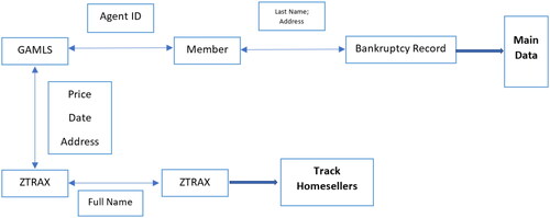
Our data mainly come from three resources: GAMLS, bankruptcy records, and ZTRAX data. We give detailed information regarding the three datasets and present how we match them together.

3.4.1. GAMLS Data

We get MLS data in Georgia from GAMLS.com. GAMLS data includes all houses listed in GAMLS.com whether they were sold or not. We have property physical characteristics in the hedonic model, such as address of the property, house and lot size, number of bedrooms and bathrooms as well as listing information, such as listing date, listing price, sale price, closing date, and time on market. Most importantly, the data contain broker information, such as name, agent ID (coded in GAMLS system), and firm where they work. Following Rutherford et al. (2005), we mainly focus on the agency problem between the listing agent and home sellers since the listing agent is more likely to determine how much the house is listed for at the beginning of the home selling process, how much the house is sold for at the end of home selling process and how long the house stays on the market. We keep single-family detached homes listings with a valid real estate agent name from January 1, 2000 to October 1, 2020.

3.4.2. Bankruptcy Records

We obtain personal bankruptcy filing records from the Georgia Northern Bankruptcy Court in the Public Access to Court Electronic Records (PACER) system. While there are three bankruptcy districts in Georgia, we only get a fee-exemption access to the Georgia Northern Bankruptcy Court in the northern districts as depicted in Figure 1. Although our sample only covers one of three districts in Georgia, we argue that the bankruptcy filings in the Georgia Northern Bankruptcy Court are representative since the counties with the most personal bankruptcies (Fulton, Dekalb, and Gwinnett) are all located in this district. Most importantly, the district includes the Atlanta housing market, where most real estate agents are located and most housing transaction activities in Georgia occur.

Figure 1. Northern District of Georgia. Notes: This figure shows the cities in the Northern District of Georgia (NDGA), where we have fee-exemption access to personal bankruptcy data. The district includes four cities: Atlanta, Rome, Newnan, and Gainesville. The gray area denotes the middle and southern districts of Georgia.

Bankruptcy data contains filer information including debtor’s name and home address as well as case information including filing date from January 1, 2000, to November 30, 2020, chapter type, creditor name, and so forth. We also complement our bankruptcy record filings from PACER with the Integrated Bankruptcy Database (IDB)¹¹ to get the income and debt amount information of each bankruptcy case. We link these two datasets with a unique identifier: case number.

3.4.3. ZTRAX Data

We use the Zillow Transaction and Assessment Dataset (ZTRAX) from January 1, 2000, through August 1, 2020, which contains two main parts: the assessment record and the transaction record. In the transaction record, we have transaction information such as transaction price, transaction time, non-arm’s-length transaction indicator,¹² mortgage information (cash sales or financed by mortgage, as well as the amount of the mortgage), buyer’s name, and seller’s name. The assessments record is originally generated by the county assessor’s office and contains physical characteristics of houses including the property type (e.g., single-family houses, condominiums), house size (gross living area in square feet), lot size in square feet, property age based on the year built, occupancy status (e.g., owner-occupied or investment), garage, and location.¹³ The transaction and tax assessment records are joined by the parcel ID. We only keep single-family or inferred single-family houses transactions in Georgia.

3.4.4. Matching across Different Datasets

Figure 2 shows the logic of how we merge the three datasets. We first describe how we merge the GAMLS listing data to bankruptcy files. The challenge of the merge is that there is no common field or unique ID between those two datasets for us to link. We take advantage of real estate member data from GAMLS.com. That data contain information about all real estate agents registered in GAMLS, such as license number, first and last name, and firm where they work. Most importantly, it has the home address information of real estate agents. We match the GAMLS data with real estate member data according to the unique identifier, AgentID. After matching, we get GAMLS-member data, which contains both listing information and real estate agent information. Then, we match the GAMLS-member data to bankruptcy record data based on the methodology from Maturana and Nickerson (2020). We exactly match zip code, street number of the address, and last name between GAMLS-member and bankruptcy record data. Our main analysis relies on this GAMLS-member-bankruptcy merged data.¹⁴

Figure 2. Linkage among three datasets. Notes: The figure shows the data linkage among three datasets: GAMLS listing data, personal bankruptcy filing data and ZTRAX data. First, we merge the GAMLS listing data to bankruptcy files by taking advantage of Member data. We call this merged dataset GAMLS-member-bankruptcy data, which is used for our main regression. Second, we also merge the GAMLS listing data with the transaction data from ZTRAX based on sale price, sold date, and address of the property. The matched dataset is called GAMLS-ZTRAX data, which is used for identifying which home sellers’ houses are represented by financially distressed brokers. Third, we match seller name and buyer name within ZTRAX data to track the home sellers’ purchase activity following Buchak et al. (2020).

Next, we describe how we merge the GAMLS listing data to the transaction data from ZTRAX. The listing data contain the property’s street address, ZIP code, closing date (the date when the home buyer and home seller completed the transaction), transaction price, property type, number of bedrooms, and number of bathrooms of each listing. However, GAMLS does not have the buyer’s name or seller’s name, which are used to track individuals’ purchase decision and mobility over time. The transaction data from ZTRAX contain the property’s street address, recording date, transaction price, buyer’s name, and seller’s name, but does not have agent information or listing information. The address in the transaction data from Zillow is standardized, since Zillow directly gets the data from a county office. In contrast, the GAMLS data does not have a clean and standardized address format since the information in GAMLS is manually entered by a listing agent. To overcome this problem, we formalize the address in GAMLS and parse it into street number, street name, and ZIP code. We do same thing for ZTRAX data. Then, we use the join-by match method to match listing data with the ZTRAX data based on street number, street name, and ZIP code. To ensure our match is accurate and precise, we only keep the unique matches meeting two restrictions: First, the difference in the sold price from the two datasets is less than $500, and the difference in the sold date (close date in GAMLS and recording date in ZTRAX) is less than 1 month. The matched dataset is called GAMLS-ZTRAX data. By merging those two datasets, we can identify which home sellers’ houses are represented by financially distressed agents and which are not.

Finally, we track the purchase activity of home sellers following Buchak et al. (2020). First, we extract the unique seller names as well as unique buyer names from transaction records between January 2000 and May 2020 from ZTRAX¹⁵ in each city (Atlanta, Rome, Newman, and Gainesville). Second, we start with seller names in the year 2000 by each city. We match the seller name to the buyer name in the current year and in the subsequent year (e.g., buyer name in year 2000 and in year 2001) to check if home sellers buy a house within two years after the sale. We use exact matches in the last name and fuzzy matches¹⁶ in the first name. We continue doing this until we reach the year 2020, and refer to this sample as ZTRAX-Track. Once we have this matched sample, we can track and compare the second home purchasing decisions among home sellers represented by different agents. Our analysis on the spillover effect from financially distressed agents to home sellers is based on this ZTRAX-Track data, and we compare the subsequent home purchasing decisions among home sellers represented by different agents.

3.4.5. Final Sample

Our main analysis is based on GAMLS-member-bankruptcy merged data. We identify 1,575 real estate agents who filed for bankruptcy in total as the treated sample. We plot the distribution of the personal bankruptcy filings of real estate agents each year in Appendix Figure A1, and we also include the total number of personal bankruptcy filings of all people in the Northern District of Georgia (NDGA) as a comparison. Before the financial crisis, real estate agent filings show a similar trend compared with filings in NDGA. On the contrary, real estate agents have a larger increase in personal bankruptcy filings than all people during the financial crisis. After the crisis, we observe that bankruptcy filings in NDGA and real estate agent filings produce similar trends again. Then we carefully design the control group with several steps. First, each real estate agent in our treated sample is matched with real estate agents who are not in the bankruptcy record, but who reside in the same ZIP code as the treated sample so that we ensure our sample is facing the same local economy conditions. Second, to account for heterogeneity of real estate agents, such as listing experience, we further let real estate agents in the control group carry similar listings to each treated real estate agent in the past three years before the bankruptcy filing date.¹⁷ In other words, this control group comprises real estate agents who are exposed to the same local economic conditions as the treated group, with similar listing experience. Lastly, due to concerns that some real estate agents have other primary occupations, as mentioned by Barwick and Pathak (2015), we only keep agents with at least 1.5 listings and purchases per year.¹⁸ Finally, we get 18,920 real estate agents as control matched with 1,575 treated real estate agents. This matched sample allows us to enrich our specification by not only comparing similar real estate agents, but also including agents’ ZIP code by year fixed effects that absorb any unobserved time-varying regional shocks.

We apply several data-screening steps to clean the raw data. First, since our focused outcome variable is the sale price, we only keep properties that are successfully sold, while any properties that fail to sell are removed. Second, observations with any missing values are removed. Third, to reduce the influence of outliers, properties with listing price, sale price, housing size, and lot size below the 1% or above the 99% percentiles as well as those with time on market (TOM) and property age above the 99% percentile of their corresponding levels are also removed. Lastly, after excluding fixed effect singletons, our final regression sample consists of 242,208 sold properties. Table 2 provides the summary statistics of the sample. The average sale price in our sample is $223,445, higher than the median sale price of $184,000, which indicates that the distribution of sale price is right skewed. The average listing price is $232,092, and it shows the same distribution as the sale price. The mean value of time on market (TOM) is 100 days, meaning that a typical home stays on the market for about 15 weeks before selling. A typical property has four bedrooms and two bathrooms. The average property age is 21 years, and the average house size is 2,328 square feet. Furthermore, we also report the summary statistics relating to the total number of transactions per year that each agent closed, each financially distressed agent closed, as well as each non-financially distressed agent closed. A typical agent closes 7.01 average transactions per year. We note that, on average, agents who experienced financial distress have slightly lower sales per year (6.56 transactions per year) compared to those who have never filed for bankruptcy (7.12 transactions per year) during the sample period. We include agent fixed effects to control for such agent-level specific characteristics.

Table 2. Summary statistics.

VarName	Obs	Mean	SD	Median
Sales price	242,208	223,445	146,253	184,000
Listing price	242,208	232,092	163,077	188,900
TOM	242,208	100	69	80
Beds	242,208	4	1	4
Baths full	242,208	2	1	2
Age	242,208	21	20	15
House size	242,208	2,328	1,026	2,110
Lot size	242,208	31,454	53,945	17,424
#Transactions: all agents	20,495	7.01	6	7.24
#Transactions: distressed agents	1,575	6.56	6	7.36
#Transactions: non-distressed agents	18,920	7.12	6	7.20

Note: This table provides the summary statistics of the main variables for the sold sample used in this paper. Sales price is the dollar price of a realized housing transaction. Listing price is the dollar price when the property is listed on MLS. TOM (time on market) is how long a property stays on the market before the property gets sold. Beds and Baths denote the number of bedrooms and bathrooms for a property. Age equals the year of the transaction date minus the year built, displayed in years. House size and lot size describe the size of property living areas and lot, displayed in square feet. We also provides summary statistics for the total the number of transactions each agent closed per year at the agent level.

4. Research Design and Results

4.1. Empirical Design

The key feature of our empirical setting is that we explore the timing of filing for personal bankruptcy to proxy for the timing of personal financial distress. In addition, we can observe an agent’s performance repeatedly, which enables us to exploit variations within a real estate agent over time by testing the difference in performance surrounding the distressed year. To rule out the possible concern that the results are driven by time-varying local factors,¹⁹ we also include agents’ ZIP code by year fixed effects to control unobserved time-varying local economic factors. Therefore, we can compare real estate agents who are financially distressed to those who are not in distress in the same location and at a same point of time.

We adopt a difference-in-difference approach and estimate the following equation: (1) $${\mathit{\text{Outcome}}}_{i,j,t}=\beta \times \mathit{\text{if}}\left({\mathit{\text{Distress}}}_{i,t}\right)+{\theta }_i+{\delta }_{a,t}+X_j+{\gamma }_{m,t}+{\epsilon }_{i,j,t}$$(1)

Our observation unit is at the agent(i)-property(j)-year(t) level. Our main outcome variable of interest is the sale price of clients’ houses. The primary independent variable we are interested in is $\mathit{\text{if}}\left({\mathit{\text{Distress}}}_{i,t}\right)$ which equals to 1 if agent i in year t files for bankruptcy, and 0 otherwise.²⁰ The coefficient of dummy variable $\mathit{\text{if}}\left({\mathit{\text{Distress}}}_{i,t}\right),$ $\beta ,$ measures the average effect of personal financial distress on performance in the treated group relative to the control group at the year of financial distress. We control for individual fixed effects, ${\theta }_i,$ to make sure our comparison is within individuals. And we add agents’ location (ZIP code) × year fixed effects to eliminate time-varying local confounding factors. We observe the characteristics $X_j$ of each property and add those as controls.²¹ Finally, we control for property market (property county) by transaction year fixed effects ${\gamma }_{m,t}.$

To see the dynamic impact of personal financial distress on real estate agents’ performance, we add different leads/lags of $\mathit{\text{if}}\left({\mathit{\text{Distress}}}_{i,t}\right)$ and estimate following regression: (2) $${\mathit{\text{Outcome}}}_{i,j,t}={\beta }_t\times \sum _{t=-4}^3\mathit{\text{if}}\left({\mathit{\text{Distress}}}_{i,t}\right)+{\theta }_i+{\delta }_{a,t}+X_j+{\gamma }_{m,t}+{\epsilon }_{i,j,t}$$(2) where year 0 indicates the exact year when the real estate agent filed for bankruptcy, year1 indicates the year prior to the bankruptcy filing, and year-2 indicates two years before the filing date, etc. The coefficient on the interaction term, β_t, captures the differences between treated and control at the different points in time relative to agents’ distress event. This design allows us to check the parallel trend between two groups before the financial distress and allows for the understanding of the dynamic path of the impact of personal financial distress on performance over time.

4.2. Baseline Result

We mainly discuss the impact of personal financial distress on performance with sale price as an outcome variable. Table 3 presents the regression results from Equation (1)(1) $${\mathit{\text{Outcome}}}_{i,j,t}=\beta \times \mathit{\text{if}}\left({\mathit{\text{Distress}}}_{i,t}\right)+{\theta }_i+{\delta }_{a,t}+X_j+{\gamma }_{m,t}+{\epsilon }_{i,j,t}$$(1) under different controls. In Column (1), we add agent fixed effects, year fixed effects, and all housing characteristics as controls, and the result shows that the sale price of client’s house drops by 5.3%, on average, in the year when the house is represented by a real estate agent who are in a distressed year than non-distressed year, compared with the control group. This large magnitude may be driven by time-varying agent location or property location factors. Therefore, we separately add agents’ location × year fixed effects and property market (county) × year and year-quarter fixed effects, and the magnitude drops as Columns (2) and (3) show. Column (4) shows the result with all controls. The sale price of agent-represented houses falls by 4% in the year when real estate agents are financially distressed from the value in the non-distressed year, relative to the control group. Relative to the mean, the sale price of clients’ houses drops by $8,938 when represented agents who are financially distressed.

Table 3. Impact of personal financial distress on sales price.

Dep.Var	ln(Sales price)
	(1)	(2)	(3)	(4)
if (Distressi,t)	−0.053***	−0.037**	−0.056**	−0.040***
	(−3.22)	(−2.30)	(−2.24)	(−2.60)
Baths	0.113***	0.111***	0.106***	0.105***
	(29.58)	(28.92)	(28.90)	(28.38)
Beds	0.003	0.002	0.000	0.001
	(1.14)	(1.02)	(0.23)	(0.28)
Age	−0.009***	−0.010***	−0.011***	−0.011***
	(−29.12)	(−31.16)	(−37.28)	(−38.64)
Age^2	0.000***	0.000***	0.000***	0.000***
	(23.47)	(24.20)	(27.34)	(28.11)
ln(House size)	0.666***	0.665***	0.642***	0.641***
	(101.80)	(104.38)	(103.22)	(104.84)
ln(Lot size)	0.045***	0.047***	0.063***	0.065***
	(20.61)	(22.04)	(32.90)	(34.61)
Agent individual FE	Yes	Yes	Yes	Yes
Year FE	Yes	No	No	No
Agent location × year FE	No	Yes	No	Yes
Housing market × year FE	No	No	Yes	Yes
N	242,208	242,208	242,208	242,208
R^2	0.771	0.782	0.790	0.799

Note: His table shows the regression results of the impact of personal financial distress on real estate agents’ performance. The dependent variable is ln(Sales Price). The independent variable we are interested in is dummy variable if(Distress). Column (1) gives our result with agent individual fixed effects and year fixed effects separately. Column (2) gives our result with agent individual fixed effect and Agent Location by Year fixed effects. Column (3) gives a result with agent individual fixed effects and Property Market by Year fixed effects. Column (4) gives a result with agent individual fixed effects, Agent Location by Year fixed effects, and Property Market by Year fixed effects. Agent Location is the ZIP code where the real estate agents live. Property Market is the county where agents’ represented houses located. *, **, and *** denote statistical significance at the 10, 5, and 1 percent levels, respectively. Standard errors are clustered at the individual level.

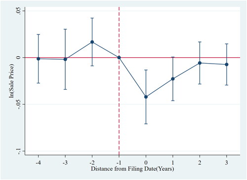
We also test the timing of the negative effect of personal financial distress on sale price. We construct different leads and lags indicators to capture the performance dynamic around the timing of personal financial distress, as Equation (2)(2) $${\mathit{\text{Outcome}}}_{i,j,t}={\beta }_t\times \sum _{t=-4}^3\mathit{\text{if}}\left({\mathit{\text{Distress}}}_{i,t}\right)+{\theta }_i+{\delta }_{a,t}+X_j+{\gamma }_{m,t}+{\epsilon }_{i,j,t}$$(2) shows. From this equation, we identify at which point in time personal financial distress has a significant impact on outcomes. We plot the estimated coefficient, β_t, from Equation (2)(2) $${\mathit{\text{Outcome}}}_{i,j,t}={\beta }_t\times \sum _{t=-4}^3\mathit{\text{if}}\left({\mathit{\text{Distress}}}_{i,t}\right)+{\theta }_i+{\delta }_{a,t}+X_j+{\gamma }_{m,t}+{\epsilon }_{i,j,t}$$(2) with the corresponding confidence intervals. Figure 3 shows the dynamic regression results for sale price. The insignificant coefficient prior to the event validates our parallel trend assumption, and the significant and negative effect is limited to the year when agents are financially distressed. The insignificant results before distress also indicate that the result is not driven by the heterogeneity in real estate agents’ quality related to personal financial distress. We also observe a reverse trend of this effect on performance, which further indicates that the effect from personal financial distress is only pronounced in the year of financial distress and that this effect gradually diminishes in the following year after the distress. It should be noted that although the financial distress leads up to personal bankruptcy, we do not think distressed status already exists one year prior to the bankruptcy filing date as those filing bankruptcy must take a credit counseling course 180 days or less before filing according to the law,²² which could potentially explain why the results are not significant one year prior to the filing date. Also, bankruptcy filings usually take about four to six months to be settled. As such, the filing year used in our baseline and 6-month-range in our robust tests can largely capture the distressed periods.

Figure 3. Dynamics of the impact on sale price. Notes: The figure shows the coefficient plot from a DID regression (along with 95% confidence intervals). The dependent variable is ln(Sales Price). The variable we are interested in is lead/lags of if(Distress). Year 0 indicates the exact year when the real estate agent filed for bankruptcy, year-1 indicates the year prior to the bankruptcy filing, year -2 indicates two years before the filing date, etc.

One question that remains unclear is why the owners accept a lower selling price as well as the loss caused by distressed agents. As pointed out by Rutherford et al. (2005) and Levitt and Syverson (2008), home sellers typically have limited knowledge about the intricacies of the real estate market, including current market conditions, comparable property values, and effective pricing strategies. Moreover, home sellers possess less knowledge and less expertise regarding the real estate market than does a real estate agent. The resulting information asymmetry can create a situation where homeowners heavily rely on their agents for advice, guidance, and pricing recommendations, which could potentially make sellers accept an offer that may be in the best interest of the agent (Levitt & Syverson, 2008).

4.3. Explanations for Results

We explain the results by referring to the literature on behavior research. Behavioral economics research argues that a negative income event impacts time discounting, and makes people behave more impatiently when making financial decisions.

In our setting, personal financial distress makes real estate agents less patient for monetary rewards, which leads to the decrease in time spent on housing-search-related tasks, which further leads to a lower sale price. If this explanation is correct, we may see financially distressed agents may want to list clients’ houses at a lower price and close the deal as quickly as possible. To test this hypothesis, we estimate Equation (1)(1) $${\mathit{\text{Outcome}}}_{i,j,t}=\beta \times \mathit{\text{if}}\left({\mathit{\text{Distress}}}_{i,t}\right)+{\theta }_i+{\delta }_{a,t}+X_j+{\gamma }_{m,t}+{\epsilon }_{i,j,t}$$(1) by replacing outcomes with listing price and TOM and report the regression results in Table 4.

Table 4. Explanation of the results.

	ln(Listing price)	ln(TOM)	ln(Sales price)
Dep.Var	(1)	(2)	(3)	(4)	(5)
if (Distressi,t)	−0.036**	−0.141***	−0.027***	−0.038***	−0.024**
	(−2.46)	(−6.81)	(−2.71)	(−2.60)	(−2.39)
ln(Listing price)			0.410***
			(18.60)
If(Downward change)				−0.003***
				(−13.48)
ln(TOM)					0.023***
					(11.80)
Housing attribute	Yes	Yes	Yes	Yes	Yes
Agent individual FE	Yes	Yes	Yes	Yes	Yes
Agent location × year FE	Yes	Yes	Yes	Yes	Yes
Housing market × year FE	Yes	Yes	Yes	Yes	Yes
N	242,208	242,208	242,208	242,208	242,208
R^2	0.806	0.351	0.875	0.799	0.876

Note: This table shows the regression results for the explanation of our main results. The dependent variable is ln(Listing Price) in Column (1), ln(TOM) in Column (2), and ln(Sales Price) in Columns (3)–(5). Columns (3)–(5) show the analysis on the decomposition of sale price discount, i.e., how much sale price discount can be explained by initial listing price in Column (3), downward changes in listing price (if the listing price decreases before the property is sold) in Column (4), and TOM in Column (5), respectively. The independent variable we are interested in is the dummy variable if(Distress). We add housing attributes as well as agent individual fixed effects, Agent Location by Year fixed effects, and Property Market by Year fixed effects. *, **, and *** denote statistical significance at the 10, 5, and 1 percent levels, respectively. Standard errors are clustered at the individual level.

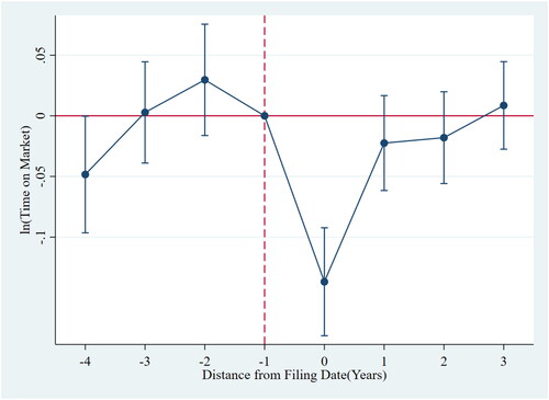
Table 4 Column (1) shows that the listing price decreased by 3.6% offered by the real estate agents in the distressed year than non-distressed year, compared with those listings provided by non-financially distressed agents, which indicates that personal financial distress makes real estate agents less likely to list clients’ property at a higher price. Relative to the mean, the price of clients’ houses listed by distressed agents drop by $8,355. Column (2) shows that the TOM of houses represented by distressed agents also drops, which implies real estate agents are more likely to close the deal sooner when facing a negative financial event. Relative to the mean, clients’ houses stay on the market 14 days longer if represented by agents who are financially distressed. We also re-estimate equation (2) and plot the coefficient in Figures 4 and 5. Both figures behave similarly to sale prices and indicate that the significant and negative effect only shows up in the year when agents are financially distressed.

Figure 4. Dynamics of the impact on listing price. Notes: The figure shows the coefficient plot from a DID regression (along with 95% confidence intervals). The dependent variable is ln(Listing Price). The variable we are interested in is lead/lags of if(Distress). Year 0 indicates the exact year when the real estate agent filed for bankruptcy, year-1 indicates the year prior to the bankruptcy filing, year-2 indicates two years before the filing date, etc.

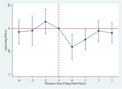
Figure 5. Dynamics of the impact on TOM. Notes: The figure shows the coefficient plot from a DID regression (along with 95% confidence intervals). The dependent variable is ln(Time on Market). The variable we are interested in is lead/lags of if(Distress). Year 0 indicates the exact year when the real estate agent filed for bankruptcy, year-1 indicates the year prior to the bankruptcy filing, year-2 indicates two years before the filing date, etc.

We implement another test to decompose the sale price discount and explore how much of it can be explained by the initial listing price, changes in the listing price, and TOM, respectively, by adding each of them as control variables to see how the coefficients change compared with the baseline result in Column (4) of Table 3. We start by adding the listing price as an additional control, and Column (3) of Table 4 finds that the coefficient drops to 2.7%, which indicates around 32.5% (1–2.7%/4.0%) of the sale price discount in the baseline is explained by the initial listing price. Furthermore, as presented in Columns (4) and (5), 5.0% and 40% of the discount in the baseline is explained by downward changes in listing prices and TOM, respectively.

Some argue that financially distressed agents may want to increase the total number of sales by decreasing the sale price. To test this hypothesis, we estimate Equation (1) with the sale probability, total number of listed and sold houses as outcomes. Columns (1) to (4) in Appendix Table A4 Panel A indicate that personal financial distress does not significantly increase sale probability as well as total number of listed and sold houses.

In sum, our results find that personal financial distress makes real estate agents less patient for monetary reward, and cause agents to sell clients’ houses quickly at a lower price. Financially distressed agents sell clients’ houses for $8,938 less but close the deal two weeks earlier than non-distressed agents. In other words, distressed agents forgo around $268 in commission compared to non-distressed agents, but received the $6,435 commission two weeks earlier.²³ We do not find evidence that agents are trying to increase the probability of sale or number of total sales when experiencing distress.

4.4. Robustness Tests

We perform several robustness tests to be sure the negative effect on real estate agents’ performance is driven by personal financial distress rather than other confounding factors.

4.4.1. Reverse Causality

We are concerned that bankruptcy filing may be endogenously determined by the decline of housing prices and that there exists a reverse causality. We implement a subsample test and restrict the sample to agents whose represented houses are located in areas with an increasing home price index (HPI) prior to the agents’ bankruptcy filing. Column (1) in Table 5 Panel A show that a significant and negative result is still present, which suggests that reverse causality does not drive our results.

Table 5. Robustness tests.

Panel A: Robust test with subsamples.
		ln(Sales price)
	Increasing	Ex same	Ex same	Listed before/Sold	Keep full name
	HPI	ZIPs	Counties	After filings	Matched
Dep.Var	(1)	(2)	(3)	(4)	(5)
if (Distressi,t)	−0.029**	−0.038**	−0.066***	−0.023**	−0.043***
	(−1.99)	(−2.51)	(−3.25)	(−2.01)	(−2.59)
Housing attribute	Yes	Yes	Yes	Yes	Yes
Agent individual FE	Yes	Yes	Yes	Yes	Yes
Agent location × year FE	Yes	Yes	Yes	Yes	Yes
Housing market × year FE	Yes	Yes	Yes	Yes	Yes
N	150,765	198,950	123,455	6,090	222,805
R^2	0.800	0.792	0.799	0.575	0.783
Panel B: Decompose agents’ bankruptcy filings
	(1)	(2)	(3)	(4)
	if (Distressi,t)	ln(Sales price)	ln(Listing price)	ln(TOM)
Residualsit		−0.032**	−0.028**	−0.132***
		(−2.32)	(−2.24)	(−5.51)
ΔHPI(agent location)i,t-1	−0.040***
	(−9.12)
ΔHPI(seller location)i,t-1	−0.046***
	(−18.84)
Housing attribute	–	Yes	Yes	Yes
Agent individual FE	–	Yes	Yes	Yes
Agent location × year FE	–	Yes	Yes	Yes
Housing market × year FE	–	Yes	Yes	Yes
N	106,542	242,208	242,208	242,208
R^2	0.003	0.799	0.805	0.214
Panel C: Robustness test with fixed effects.
	ln(Sales price)
	Repeated sales	Same sellers	Same firms
Dep.Var	(1)	(2)	(3)
if (Distressi,t)	−0.049***	−0.079*	−0.030**
	(−2.67)	(−1.80)	(−2.14)
Housing attribute	Yes	Yes	Yes
Agent individual FE	Yes	Yes	Yes
Agent location × year FE	Yes	Yes	Yes
Housing market × year FE	No	Yes	Yes
Property FE	Yes	No	No
Seller FE	No	Yes	No
Office FE	No	No	Yes
N	234,189	113,374	94,724
R^2	0.985	0.992	0.804
Panel D: Another source of personal distress-decline in personal housing wealth.
	Δln(Sales price)	Δln(Listing price)	Δln(TOM)
Dep.Var	(1)	(2)	(3)
ΔHPI	0.459***	0.515***	0.811***
	(3.53)	(4.01)	(7.85)
Agent Location × housing market, year	Yes	Yes	Yes
N	9,958	9,958	9,958
R^2	0.317	0.328	0.129

Note: This table shows the robustness tests of the impact of personal financial distress on sale price. In Panel A, Column (1) shows the results when we restrict the sample to agents whose represented houses are located in areas with increasing housing price index (HPI) prior to filing for bankruptcy. Columns (2) and (3) show the results when we restrict the sample to the properties located at different ZIP codes/counties from where the real estate agents live. Column (4) presents the results when we limit sample to the houses are listed before represented agents’ bankruptcy and sold out after the bankruptcy. Column (5) shows the results when we keep agents whose full names are exactly matched with the bankruptcy record. Panel B shows the results of two-stage regressions. At the first stage, the dependent variable is the likelihood of personal financial distress each year at each individual agent level and independent variables are the one-year lagged changes in home price index (HPI) in both the agents’ location and the home seller’s locations (i.e., average house price index changes in the region where agents’ represented houses are located), and Column (1) presents the results. At the second stage, the three main outcome variables include sale price, listing price, and TOM and the main explanatory variable is the residuals from the first-stage regression, and the results are illustrated across Columns (2) to (4). In Panel C, Columns (1) to (3) show the results when we add property fixed effects (Housing Attribute only includes the property age), seller fixed effects and firm fixed effects. Panel D shows the results for another source of personal financial distress. *, **, and *** denote statistical significance at the 10, 5, and 1 percent levels, respectively. Standard errors are clustered at the individual level.

4.4.2. Unobserved Local Shocks to Sale Price

In the baseline regression, we add agents’ ZIP code by year fixed effects to control time-varying local economics which may drive both a higher likelihood of distress as well as a decline in performance. There may remain concerns that ZIP code by year fixed effects are not granular enough to control for unobserved local confounding factors. To further determine if our results are driven by the local economy, we exclude properties located in the same ZIP codes or counties as where the real estate agent lives. Columns (2) through (3) in Table 5 Panel A again show similar results, which helps rule out the possibility that more granular local factors drive our results.

4.4.3. Decomposition of Agents’ Bankruptcy Filings

Furthermore, we take an additional step to address the concern that the decision to file for bankruptcy by agents may be influenced by market conditions that may contribute to the underperformance of sales outcomes. In other words, there is a possibility that both the sales outcome and likelihood of personal bankruptcy filings are influenced by a decline in home prices within the same region. In response, we conduct a series of two-stage regressions. Specifically, we first implement a regression of the likelihood of experiencing personal financial distress each year at each individual agent level on the one-year lagged changes in the home price index (HPI) in both the agent’s location and the home seller’s location. The purpose of conducting the first stage is to disentangle agents’ bankruptcy filings into two components: one driven by local market conditions (predicted) and the other influenced by more exogenous factors (residuals). We then use sale price, listing price, and TOM as dependent variables with the residuals as the explanatory variable in the second stage from the first regression.

The regression results are presented in Panel B of Table 5. As shown in Column (1), the two variables—the one-year lagged changes in home prices in the agent’s location and in the home seller’s location—are significantly and negatively associated with the likelihood of personal financial distress in the current year. We then estimate a regression with three outcome variables: sale price, listing price, and TOM on the residuals calculated based on Column (1). Columns (2)–(4) show that the negative and significant results remain if using residuals as the explanatory variable instead, which assures us that our baselines are less likely to be completely driven by endogenous market conditions.

4.4.4. Selection Bias

There may exist a selection bias or sorting issue. Bankrupt real estate agents may have a higher likelihood to get worse properties to sell with lower profit margins and match with clients who have lower reservation housing prices.

To begin with, some may suggest the explanation for the negative effect of personal financial distress on sale price is that agents may target houses with lower intrinsic value when they are financially distressed. In another words, some unobserved housing characteristics may drive our results. To test this hypothesis, we use a repeated-sale approach and restrict the sample to the properties with repeat sales only. We add property fixed effects in the regression to control for time-invariant property characteristics, and Column (1) in Table 5 Panel C show the effect still remains.

Furthermore, some may be concerned that financially distressed agents may choose clients or firms who are willing to sell houses at a lower price. The difference in sale price may simply reflect the heterogeneity in client or firm characteristics. For example, financially distressed agents may intend to target impatient sellers so that they can sell the houses quickly or firms where real estate agents are working may prefer to list and sell houses with different prices. To test this hypothesis, we link the GAMLS data to ZTRAX data to get the sellers’ information. We only keep those sellers who appear multiple times according to the name, which indicates they sell multiple properties following Barwick et al. (2017). We add seller fixed effects to control for seller attributes, and the regression results are reported in Column (2). We still obtain significant and negative results, which rules out the possibility that seller’s preferences drive our results. Similarly, we add the firm fixed effects to control for the time-invariant quality of firms. We find a similar negative effect of personal financial distress on sale price when comparing within the same firm, as Column (3) show.

Moreover, we are concerned that if the owner is indeed aware of the agent’s bankruptcy and avoids such agents, the current results cannot be fully interpreted as an effect of the bankruptcy on the agent’s performance. Thus, there could exist a potential selection issue. Specifically, the home represented by the bankrupt agent may be of low value because the reputation of the bankrupt agent is damaged as a result of the bankruptcy, whereas the seller of a high-value home is not interested in finding a bankrupt agent. To account for this potential effect, we conducted a subsample test and include a subsample in which the houses are listed before a represented agent’s bankruptcy and sold after the bankruptcy to check if the results change. As illustrated in Column (4), Panel A of Table 5, we find that the negative and significant results still exist, which alleviates the concerns mentioned above.

Lastly, we have a concern that our analysis might be subject to survivorship bias if financially distressed agents are more likely to exit the sample. We construct a dummy variable I(exit_i,t), which takes on the value of 1 if Agent i exits the sample at time t, and we compare the exit rate of the financially distressed agents versus non-distress agents before and after the bankruptcy filing. Appendix Table A4 Panel B reports the result, and the insignificant coefficient on $\mathit{\text{if}}\left({\mathit{\text{Distress}}}_{i,t}\right)$ indicates the exit rate for agents does not experience a higher increase after the bankruptcy filing. One possible explanation is that our sample is limited to full-time agents for whom the commission is their primary source of income; therefore, they may have to work as an agent to make a living even when facing financial distress instead of exiting the market completely.

4.4.5. Another Source of Personal Financial Distress: Decline in Housing Wealth

Finally, some may still be concerned that unobserved time-varying factors at the individual level could drive our results. We have a concern that our test does not preclude all possibilities of another correlated omitted variable. For example, Maturana and Nickerson (2020) mention that omitted variables such as health shock, or divorce, in the context of personal bankruptcies can have an adverse impact on the estimate. While we do not have access to filers’ health or divorce information, we explore another source of personal financial distress, which is the decline of personal real estate wealth to further establish a causal relation between personal financial distress and agents’ performance. Following Pool et al. (2019) and Bernstein et al. (2021), we use variation in the severity of the financial crisis in 2008 and afterwards to create exogenous changes (decline) in real estate agents’ wealth to proxy for personal financial distress. We estimate the following regression: (3) $${\Delta \mathit{\text{Outcome}}}_{i,\mathit{\text{hz}},\mathit{\text{pre}},\mathit{\text{post}}}=\beta \times \Delta \mathrm{\%}{\mathit{\text{HPI}}}_{i,\mathit{\text{az}},\mathit{\text{pre}},\mathit{\text{post}}}+{\theta }_{a\mathrm{c},\mathit{\text{hz}},t}+{\epsilon }_{i,\mathit{\text{hz}},t}$$(3)

We define the pre-period as 2005–2007 and the post-period as 2008–2010. As such, our sample is limited to the years between 2005 and 2010. We aggregate the outcome variables (i.e., taking the average of sale price, listing price, and time on market) into agent (i), clients’ houses ZIP code (hz) and year (t) level, and then get the difference ${\Delta \mathit{\text{Outcome}}}_{i,\mathit{\text{hz}},\mathit{\text{pre}},\mathit{\text{post}}}$ between the post-period (post) and pre-period (pre). The main variable $\Delta \%{\mathit{\text{HPI}}}_{i,\mathit{\text{az}},\mathit{\text{pre}},\mathit{\text{post}}}$ denotes the percent change in the house price index between the post-period and pre-period for agents’ location ZIP code (az), which is used as a proxy of the agents’ personal financial distress. We also add agent location (county) by represented clients’ houses location (ZIP code) by year fixed effects (${\theta }_{\mathit{\text{ac}},\mathit{\text{hz}},t}$). Therefore, we compare two agents who are living in the same county and whose represented houses are in the same ZIP code and are sold in the same year, but who face different changes in housing wealth (proxied by the house price index changes in agents’ living locations).²⁴ We expect that agents with a large decline in personal housing wealth would experience a decrease in outcome variables. Table 5 Panel D shows that a decrease in agents’ housing wealth is associated with the decrease in sale price, listing price, and time on market of the houses represented by agents. Therefore, by exploring an exogenous shock to the personal wealth of real estate agents, we further validate that personal financial distress could drive lower performance.

4.5. Additional Tests

4.5.1. Stacked DID

Recent studies on DID analysis (Baker et al., 2022; Callaway et al., 2021; Goodman-Bacon, 2021) have highlighted that two-way fixed effects models (such as staggered DID) exhibit bias and lead to inaccurate inferences. The main cause of the bias is that the estimator depends partly on a comparison between the later-treated and earlier-treated observations, with the earlier-treated ones serving as controls. To mitigate this concern, we adopt the stacked DID following Baker et al. (2022). For each filing event, we assign a clean control group to the treated group (i.e., agents who have experienced distress). The clean control group includes both (1) agents who have not yet experienced a distress event during the study period (4-year window surrounding the distressed year) for each focal distressed agents and (2) agents who never experienced a distressed event in the sample. We construct an event-specific identifier and stack together the event-specific datasets. We then estimate the stacked regressions and control for interactions between the previously used fixed effects and filing events fixed effects. As seen in Table 6 Panel A, our main results are qualitatively similar when we use the stacked DID method.

Table 6. Additional tests.

Panel A: Stacked regression.
	ln(Sales price)
	(1)	(2)	(3)	(4)
if (Distressi,t)	−0.058***	−0.040***	−0.052***	−0.042***
	(−3.12)	(−3.41)	(−3.13)	(−4.00)
Housing attribute	Yes	Yes	Yes	Yes
Agent individual × event FE	Yes	Yes	Yes	Yes
Year × event FE	Yes	No	No	No
Agent location × year × event FE	No	Yes	No	Yes
Housing market × year × event FE	No	No	Yes	Yes
N	311,420	311,420	311,420	311,420
R^2	0.803	0.811	0.832	0.843
Panel B: Impact of personal financial distress on purchase outcomes – buying agent.
	ln(Purchase price)	ln(TOM)
	(1)	(2)
if (Distressi,t)	0.021**	−0.104***
	(2.25)	(−4.21)
Housing attribute	Yes	Yes
Agent individual FE	Yes	Yes
Agent location × year FE	Yes	Yes
Housing market × year FE	Yes	Yes
N	198,313	198,313
R^2	0.714	0.762
Panel C: Simultaneous regression results-3SLS.
	ln(Sales price)	ln(TOM)
	(1)	(2)
if (Distressi,t)	−0.044***	−0.143***
	(−2.71)	(−2.62)
ln(TOM)	0.045***	–
	(2.59)	–
ln(Sales price)	–	14.045***
	–	(2.87)
Listing density	−0.005**	–
	(−2.26)	–
Competition	–	0.029***
	–	(2.94)
Housing attribute	Yes	Yes
Agent individual FE	Yes	Yes
Agent location × year FE	Yes	Yes
Housing market × year FE	Yes	Yes
N	242,208	242,208
R^2	0.774	0.325
Panel D: Heckman regression results-2SLS.
	Dummy(sold)	ln(Sales price)
	(1)	(2)
Markup	−0.573***
	(−3.94)
if (Distressi,t)		−0.039***
		(−2.62)
Inverse mills ratio		0.045***
		(2.58)
Housing attribute	Yes	Yes
Agent individual FE	Yes	Yes
Agent location × year FE	Yes	Yes
Housing market × year FE	Yes	Yes
N	403,781	242,208
(Pseudo) R^2	0.032	0.843

Note: This table shows the additional tests of the impact of personal financial distress on sale price. In Panel A, the sample is constructed following the “stacked regression” approach as suggested by Baker et al. (2022). The number of observations is different from the baseline regression as we stack the sample together. Event FE is an event-specific identifier to control each filing event. In Panel B, it shows shows the results of the purchase outcomes for transactions represented by the distressed selling agents. The dependent variable is ln(Purchase Price) in Column (1) and ln(TOM) in Column (2). Panel C uses a 3SLS regression model to overcome the problem that price and TOM are simultaneously determined and Panel D adopts Heckman-2SLS to mitigate the sample selection issue. *, **, and *** denote statistical significance at the 10, 5, and 1 percent levels, respectively. Standard errors are clustered at the individual level.

4.5.2. Alternative Outcome Variables

The prior analysis focuses on the sales price and time-on-market of financially distressed agents’ listings. We explore the sales price and time-on-market of transactions where the financially distressed agent represents the buyer and we match the agents who represent the buyer to the bankruptcy records and explore the sales price as well as time-on-market for transactions where the financially distressed agent represents the buyer. Hence, we add the following sentence.

We have studied the sales outcomes of distressed agents’ listings, and in this section, we explore the purchase prices and time-on-market (TOM) of transactions where financially distressed agents represent the buyer. We match the names as well as locations of agents who represent the buyer to the lists of bankruptcy records and define 1,064 buyer’s agents who filed for bankruptcy during our sample period as the treated groups and 11,342 buyer’s agents who never filed serving as the control groups.

We now re-estimate Equation (1)(1) $${\mathit{\text{Outcome}}}_{i,j,t}=\beta \times \mathit{\text{if}}\left({\mathit{\text{Distress}}}_{i,t}\right)+{\theta }_i+{\delta }_{a,t}+X_j+{\gamma }_{m,t}+{\epsilon }_{i,j,t}$$(1) by comparing the transactions represented by the distressed versus non-distressed buyer’s agents in the distressed year relative to the non-distressed year and report Table 6 Panel B. Notably, the positive and significant coefficient in Column (1) shows there is an increase in purchase prices for houses represented by the buyer’s agents in the distressed year over the non-distressed year, compared with those houses represented by non-financially distressed buyer’s agents. However, TOM decreases when financially distressed buyer’s agents represent buyers to purchase houses. The above results suggest that when acting on behalf of the buyer, agents experiencing financial difficulties may also have lower bargaining power and are more likely to suggest paying more than for a property, which could potentially enhance the probability of finalizing the transaction and increase their commission.²⁵

4.5.3. Price and TOM Simultaneously Determined

The results from our baseline estimation may suffer a bias as the sales price and TOM are simultaneously determined. To address the potential endogeneity issues, we follow Zahirovic-Herbert and Gibler (2014) and Bian et al. (2017) to conduct 3SLS regression analysis below: (4) $${\mathit{\text{ln}}\left(\mathit{\text{Sale Price}}\right)}_{i,j,t}=\beta \times \mathit{\text{if}}\left({\mathit{\text{Distress}}}_{i,t}\right)+{\zeta \times \mathit{\text{ln}}\left(\mathit{\text{TOM}}\right)}_{i,j,t}+\eta {{\times \mathit{\text{ListingDensity}}}_{i,j,t}+\theta }_i+{\delta }_{\mathrm{a},t}+X_j+{\gamma }_{m,t}+{\epsilon }_{i,j,t}$$(4) (5) $${\mathit{\text{ln}}\left(\mathit{\text{TOM}}\right)}_{i,j,t}=\beta \times \mathit{\text{if}}\left({\mathit{\text{Distress}}}_{i,t}\right)+{\zeta \times \mathit{\text{ln}}\left(\mathit{\text{Sale Price}}\right)}_{i,j,t}+{\eta \times \mathit{\text{Competition}}}_{i,j,t}+{\theta }_i+{\delta }_{a,t}+X_j+{\gamma }_{m,t}+{\epsilon }_{i,j,t}$$(5)

Equations (1)(1) $${\mathit{\text{Outcome}}}_{i,j,t}=\beta \times \mathit{\text{if}}\left({\mathit{\text{Distress}}}_{i,t}\right)+{\theta }_i+{\delta }_{a,t}+X_j+{\gamma }_{m,t}+{\epsilon }_{i,j,t}$$(1) and (2)(2) $${\mathit{\text{Outcome}}}_{i,j,t}={\beta }_t\times \sum _{t=-4}^3\mathit{\text{if}}\left({\mathit{\text{Distress}}}_{i,t}\right)+{\theta }_i+{\delta }_{a,t}+X_j+{\gamma }_{m,t}+{\epsilon }_{i,j,t}$$(2) yield a simultaneous system where Listing Density denotes the concentration of competing listings in the neighborhood and Competition is the distance-weighted number of houses in the neighborhood that are listed on the market at the same time as the focal property, both of which serve as instrumental variables.²⁶ Table 6 Panel C reports the results of the jointly estimated price-TOM models from the simultaneous equations models (1) and (2). The sign and magnitude of the coefficient of $\mathit{\text{if}}\left({\mathit{\text{Distress}}}_{i,t}\right)$ in Columns (1) and (2) are consistent with our baseline results. These results help to alleviate the concern of the potential endogeneity issues driven by the simultaneous determination between the sales price and TOM.

4.5.4. Selection for Sold Properties

There could be a potential sample selection bias as our regression sample contains only sold properties. To address this potential issue, we employ the Heckman 2SLS (Heckman, 1979) by including both sold and unsold properties. In the first stage regression, we use markup as a potential instrumental variable, which is defined as the log difference between the initial listing price and the predicted sale price following Johnson et al. (2015) and Lin et al. (2024). In the second stage of the regression, we add the Inverse Mills Ratio (IMR) obtained from the first stage as an additional control variable. Table 6 Panel D presents the results of the Heckman 2SLS and the coefficient of $\mathit{\text{if}}\left({\mathit{\text{Distress}}}_{i,t}\right)$ is still negative and significant, which indicates sample selection bias may not drive the baseline result.

4.5.5. Different Definition of Treatment Period

In the baseline regression, our treated period is defined at the bankruptcy filing year. For example, if a person files for bankruptcy in August 2013, all of the transactions that happened in 2013 from January to December are included in the treated periods, and as such, the treated periods include months that are both before and after the filing year-month. However, there is a case where the filing events are at the beginning of each year, when the agent was clearly in financial distress at the prior year. To address such potential issues, we redefine the treated periods as transaction dates that fall into a 6-month window surrounding the filing month (6 months before and 6 months after the filing month) to fully consider the second issue. The negative and significant results in Appendix Table A2 Panel A ensure the robustness of our results.

4.5.6. Relisting Properties

We treat the relisted properties as the new listings; approximately 7% of the listings in our sample are relisted properties (we treat it as a relisting if a property was relisted within 60 days after it was taken off the market following Smith et al. (2016). Among relisted properties, around 21% changed the agent and about 17% reduced the listing prices. Smith et al. (2016) show that relisting a property results in a higher selling price. To address the concern that the relisted properties may affect our results, we drop the relisted properties and keep only new listings in our regression sample as another robustness test. The negative and significant result in Appendix Table A2 Panel B Column (4) ensures our main result is not impacted by relisted properties.

4.6. Heterogeneity Test

In this section, we want to test the heterogeneous effect of personal financial distress on the sale price based on the distress severity and the real estate market conditions to see where the agents’ financial distress has a more pronounced effect on their performance.

4.6.1. Effect across Different Distress Severity

First, we test if the negative effect of personal financial distress on sale price may vary according to agent’s distress severity. We are able to observe the characteristics of each case by linking our bankruptcy filing to the Integrated Bankruptcy Database. We have the income, total debt, and Debt-to-Income (DTI) for each case to measure distress severity, and we expect real estate agents with lower monthly income may suffer more from financial distress, and the negative effect should be more pronounced within the lower income, higher debt, and higher DTI group. To test this hypothesis, we split the sample into two groups according to the median value of monthly income, debt, and DTI and we estimate Equation (1)(1) $${\mathit{\text{Outcome}}}_{i,j,t}=\beta \times \mathit{\text{if}}\left({\mathit{\text{Distress}}}_{i,t}\right)+{\theta }_i+{\delta }_{a,t}+X_j+{\gamma }_{m,t}+{\epsilon }_{i,j,t}$$(1) with two subgroups. We find a larger and more significant impact exists in the lower income, higher debt, and higher DTI group, which confirms our expectation that real estate agents with higher distress severity suffer more from the financial events as Table 7 Panel A indicates.

Table 7. Heterogeneity test.

Panel A: Heterogeneity test on distress severity.
	ln(Sale price)
	(1)	(2)	(3)	(4)	(5)	(6)
	Income		Debt		Debt to income
Dep. Var:	Low	High	Low	High	Low	High
if (Distressi,t)	−0.068***	−0.043**	−0.036	−0.094***	−0.041*	−0.076***
	(−3.08)	(−2.00)	(−1.58)	(−4.39)	(−1.87)	(−3.80)
Housing attribute	Yes	Yes	Yes	Yes	Yes	Yes
Agent individual FE	Yes	Yes	Yes	Yes	Yes	Yes
Agent location × year FE	Yes	Yes	Yes	Yes	Yes	Yes
Housing market × year FE	Yes	Yes	Yes	Yes	Yes	Yes
N	81,782	94,492	79,685	106,188	83,178	127,983
R^2	0.79	0.798	0.792	0.796	0.798	0.796
Panel B: Heterogeneity test on housing market characteristics.
	ln(Sale price)
	(1)	(2)	(3)	(4)	(5)	(6)	(7)
	Market Cycle			Heterogeneity		Experience
Dep. Var:	Boom	Bust	Recovery	Low	High	Low	High
if (Distressi,t)	0.007	−0.094***	−0.045**	−0.011	−0.063***	−0.038***	−0.013
	(0.40)	(−3.14)	(−2.33)	(−0.69)	(−2.77)	(−3.24)	(−1.21)
Housing attribute	Yes	Yes	Yes	Yes	Yes	Yes	Yes
Agent individual FE	Yes	Yes	Yes	Yes	Yes	Yes	Yes
Agent location × year FE	Yes	Yes	Yes	Yes	Yes	Yes	Yes
Housing market × year FE	Yes	Yes	Yes	Yes	Yes	Yes	Yes
N	40,766	78,911	121,393	107,233	134,246	82,306	90,314
R^2	0.822	0.802	0.792	0.796	0.797	0.793	0.794

Note: This table shows the heterogeneity test. The dependent variable is ln(Sale Price). The independent variable we are interested in is if(Distress). Panel A shows the heterogeneity test according to agents’ distress severity, such as income, total amount of debt, and debt-to-income ratio. Panel B shows the heterogeneity test according to housing market and agents characteristics, such as market cycle, the degree of heterogeneity in local houses and selling experiences. *, **, and *** denote statistical significance at the 10, 5, and 1 percent levels, respectively. Standard errors are clustered at the individual level.

4.6.2. Effect across Different Market and Agent Characteristics

Real estate agents in different real estate market conditions may have different reactions to financial events. Table 7 Panel B Columns (1)–(3) tell us that the real estate market bust exacerbated the negative effect of personal financial distress on sale price, while the effect is negligible in the boom. We also want to see if the negative effect is stronger in a less informative environment following Agarwal et al. (2019). The estimation is presented in Table 7 Panel B Columns (4) and (5), and we find there are different impacts of personal financial distress on sale price across different degrees of heterogeneity of local houses (measured by the standard deviation of local housing prices), and real estate agents facing higher degrees of heterogeneity of local houses are more negatively affected than lower groups.

Furthermore, we conduct another heterogeneity test to analyze if the negative effect of financial distress on sales outcomes varies across agents with different listing experiences as Cunningham et al. (2022) document the importance of agents’ listing experience in the determination of the sales outcomes. We use total the number of houses sold by agents in the previous three years to measure their listing experience, then divide the sample into two groups based on the median value, and finally, re-estimate the baseline equation with two subgroups. A larger and significant effect only exists in the group with fewer listing experiences, which illustrates the agents with more listing experience mitigate the effects of personal Table 7 Panel B Columns (6) and (7) indicates.

5. Spillover Effect

We documented that the sale price of the agent-represented houses falls by 4% in the year when real estate agents are financially distressed. And since the real estate agents’ financial distress has a negative effect on the sale price of clients’ houses, this negative effect could directly spill over to home sellers through the client-agent network and lead home sellers to suffer from a loss. Since most home sellers use the proceeds from their previous house to pay for their next house, we want to study how the loss caused by financially distressed agents distorts home sellers’ purchase decisions. The data we use in this section is ZTRAX-Track data where we can track the purchase decision of a home seller following Buchak et al. (2020). We design the cross-section regression as follows: (6) $$\mathit{\text{Purchase}}\mathrm{ }{\mathit{\text{Outcome}}}_{j,m,t}=\beta \times \mathit{\text{if}}\left({\mathit{\text{Sold by distressed agent}}}_j\right)+{\gamma }_{m,t}+{\epsilon }_{j,m,t}$$(6)

Our outcome variable $\mathit{\text{Purchase}}\mathrm{ }{\mathit{\text{Outcome}}}_{j,m,t}$ includes a dummy variable indicating if the home seller j takes a loan for their second house purchase, leverage, as well as a series of dummy variables indicating if they move to a worse neighborhood after his previous house is sold at market (county) m and time t. The main variable of interest is $\mathit{\text{if}}\left({\mathit{\text{Sold by distressed agent}}}_j\right),$ which indicates whether home seller j’s previous house is sold by a financially distressed broker. In Equation (6)(6) $$\mathit{\text{Purchase}}\mathrm{ }{\mathit{\text{Outcome}}}_{j,m,t}=\beta \times \mathit{\text{if}}\left({\mathit{\text{Sold by distressed agent}}}_j\right)+{\gamma }_{m,t}+{\epsilon }_{j,m,t}$$(6) , we compare the difference of the purchase decision between the home seller represented by financially distressed brokers with those represented by financially non-distressed brokers.

To account for the possibility that owners who move to larger houses are more likely to require a loan and have a higher LTV ratio, we implement the commonly used propensity score matching (PSM) method to eliminate potential confounding factors.²⁷ Appendix Figure A2 shows the balance test results for propensity score matching and illustrates that the difference for each covariate shrinks substantially, which demonstrates a good quality of the matching for balancing the two groups. Based on this propensity score-matched (PSM) sample, Table 8 reports the regression results. Columns (1)–s(2) show that home sellers represented by financially distressed agents are more likely to use a loan and also choose a higher LTV when they purchase a similar house compared with those represented by non-distressed agents.

Table 8. Spillover effect.

	If (Loan)	LTV	I(Lower	I(Lower	I(Lower	I(Lower
			income)	education)	price)	opportunity)
Dep. Var	(1)	(2)	(3)	(4)	(5)	(6)
if (Sold by distressed agentj)	0.034**	0.032**	0.086*	0.083*	0.093**	0.084**
	(2.16)	(2.18)	(1.86)	(1.76)	(2.20)	(2.12)
Housing attribute	Yes	Yes	No	No	No	No
Housing market × year FE	Yes	Yes	Yes	Yes	Yes	Yes
N	2,832	2,832	16,892	16,892	16,892	16,892
R^2	0.756	0.682	0.057	0.069	0.046	0.054

Note: This table shows the regression results of spillover effects of personal financial distress on home sellers. The dependent variable If(Loan) in Column (1) denotes whether or not taking a loan originated to purchase next house. LTV in Column (2) denotes leverage of next home purchase. Columns (1) and (2) are based on the propensity score-matched (PSM) sample. Columns (3)–(6), I(Lower Income), I(Lower Education), I(Lower Price) and I(Lower Opportunity) are dummy variables equal to 1 if the median household income, education level (measured by the ratio of bachelors degree), median house price or the opportunity index at the new residence (ZIP code) home sellers move to is lower than the previous residence. The independent variable we are interested in is if(Sold by Distressed Agent), which takes 1 is owners’ previous houses were sold by distressed agents. *, **, and *** denote statistical significance at the 10, 5, and 1 percent levels, respectively. Standard errors are clustered at the individual level.

We also investigate if they move to a better or worse neighborhoods after home sales from Column (3) to Column (5) based on full ZTRAX-Track sample. We create three dummies to indicate the changes in neighborhoods, i.e., I(Lower Income), I(Lower Education) and I(Lower Price). The dummies equal 1 if the median household income, education level (measured by the ratio of Bachelor’s degree) or median home price at the new residence (ZIP code) home sellers move to is lower than the previous residence.²⁸ We find that home sellers whose previous house was sold by a distressed agent are more likely to move to worse neighborhoods with lower household income, lower education level and lower housing prices, which is indicated by a significant and positive coefficient from Column (3) to Column (5). There is a concern that neighborhoods with lower household income, education level, and housing price may not be truly worse off as these neighborhoods may offer other unobservable benefits. We conduct another test to examine the spillover effect, and measure if the home sellers represented by financially distressed agents are more likely to move to neighborhoods with fewer opportunities in the subsequent purchase. We leverage neighborhood opportunities from the Child Opportunity Index 2.0 (COI 2.0; Mast & Din, 2021) database and construct a dummy variable I(Low Opportunity), indicating that if the COI 2.0 score at the new residence is lower than at the previous residence.²⁹ Table 8 Column (6) shows that home sellers whose previous house was represented by distressed agents are more likely to move to the neighborhoods with fewer opportunities compared with those represented by non-distressed agents, which further validates the argument that the loss caused by financially distressed agents makes home sellers more likely to move to worse neighborhoods.

Our findings in this section highlight the spillover effect and amplification of negative events from one to another. The loss caused by distressed agents spills over to clients, and further distorts clients’ subsequent purchase decisions.

6. Conclusion

This study investigates how personal financial distress affects workers’ performance. Using the real estate brokerage industry as a setting and filing of bankruptcy as the proxy for personal financial distress, we find that sale price of the clients’ house is significantly lower in the year of filing bankruptcy, which shows that personal financial distress lowers worker’s performance. These findings are consistent with the prediction from behavioral economics research. Personal financial distress makes real estate agents want to sell a home quicker and at a lower price. The negative effect is particularly strong among real estate agents with higher debt, lower income, and higher debt-to-income ratio. Understandably, these real estate agents are more vulnerable when facing personal financial distress and more likely to be affected by negative financial events. Results also vary across different housing market conditions.

Finally, our results show the spillover effect from one to another. Most home sellers use the proceeds from a house sale to pay for their next house, and home sellers may have to distort their next house purchase decision due to the loss caused by financially distressed agents. Consistent with our conjecture, we find that home sellers are more likely to take a larger LTV and move to disadvantaged neighborhoods when their previous home was are sold by a financially distressed agent. These results highlight a negative effect of personal financial distress on performance and find the performance reduction could amplify and cause a negative spillover on clients through the agent-client network.

Disclosure statement

No potential conflict of interest was reported by the author(s).

Notes

1 In this paper, we use “client” and “home seller” interchangeably, as we do “agent” and “broker.”

2 https://www.nar.realtor/sites/default/files/documents/2020-generational-trends-report-03-05-2020.pdf.

3 This number is estimated as $246,000*5.34million*6%. We take the typical value of homes in the United States as of June 2019, which is $246,000 from Zillow and assume 6% commission fee charged for sold homes.

4 https://www.govinfo.gov/content/pkg/USCODE-2011-title11/pdf/USCODE-2011-title11-chap5-subchapII-sec525.pdf; https://www.justice.gov/osg/brief/fcc-v-nextwave-and-artic-slope-v-nextwave-brief-merits.

5 The PACER service provides electronic public access to all federal court records.

6 https://upsolve.org/learn/is-bankruptcy-discharge-public-record/; Bankruptcy filing information stays on a credit report for up to 10 years (Dobbie et al. 2020) but cannot be removed from public records.

7 To fully account for potential selection issues, we also provide more discussions in the robustness test section.

8 https://web.archive.org/web/20200404213616/https://www.bls.gov/oes/current/oes419022.htm.

9 Those ethics include but are not limited to (1) represent their client’s best interests (2) disclose all available information required by state law and (3) preserve confidential information of the client.

10 Including Alabama, Alaska, Arkansas, Colorado, Connecticut, Delaware, Florida, Kansas, Illinois, Iowa, Louisiana, Maine, Massachusetts, Mississippi, Missouri, Nebraska, Nevada, New Mexico, New Hampshire, New York, North Carolina, North Dakota, Oregon, Pennsylvania, South Carolina, Utah, Virginia, Washington, and West Virginia. The appendix provides the details of other states.

11 https://www.fjc.gov/research/idb.

12 Non-arm’s length transactions are those that happen between two individuals that have a relationship. A good example is a transaction between two family members. Normally, the transaction price in a non-arm’s-length transaction does not reflect market prices, thus we exclude all these transactions based on Zillow’s internal code.

13 Detailed variable definitions can be found in Appendix Table A1.

14 We use the last name instead of the full name to allow for the possibility that the spouse may serve as the representative for all household members when filing for bankruptcy. In our sample, 136 of 1,575 agents (8.63%) belong to the spouse filings group. Our results are robust if we only keep those matched with the full name as shown in Column (5) of Table 5.

15 The transaction record already helps us split buyer and seller names into two parts: buyer-nonindividual-name and buyer-individual-name. If it is a buyer-individual-name, it gives us first name, middle name, and last name.

16 We use the reclink command in Stata, and keep the matched score larger than 0.8.

17 The absolute value of the difference is less than 5.

18 In terms of sensitivity, we also test thresholds of 2, 2.5 and 3 transactions and find that our conclusions are not sensitive to the threshold as shown in Appendix Table A2 Panel B Column (1)–(3).

19 For example, financially distressed agents may be more likely to locate in worse areas, and local unfavorable conditions may lead to both the financial distress and lower performance.

20 Considering that agents may already be financially distressed before bankruptcy filing, our results are robust when we let if(Distress) equal 1 if the date is within 6-month ranges before and after the bankruptcy filing month.

21 In our baseline results, we add all observed attributes of the property as controls. This may reduce the number of observations. In our robustness tests, we add each attribute as a control gradually and try different specifications. Results can be found in Appendix Table A3.

22 https://www.debt.org/bankruptcy/chapter-7/how-long-does-it-take/.

23 $268 is calculated as $8,938*3% assuming the agent splits the commission. The $6,435 is calculated as $223,445*3%, minus $268.

24 Importantly, we exclude clients’ houses located in the same ZIP codes as where the real estate agent lives to rule out the possibility that local economics drive both the decline in agents’ housing wealth as well as a drop in sale price of clients’ houses.

25 We appreciate reviewer’s suggestions and comments. We do not find the personal financial distress significantly increases the total number of purchased houses for buyer’s agents, shown in Appendix Table A4 Panel A Column (5).

26 We follow Zahirovic-Herbert and Gibler (2014) and Bian et al. (2017) to construct these two variables.

27 We use the psmatch2 command in Stata, which is a standard tool used to construct PSM-matching samples. We perform a 5-nearest-neighbor matching (one-to-five matching) with replacement by using a set of home characteristics as selection determinants, including the number of bedrooms and bathrooms, age, housing size, and lot size, of the houses subsequently purchased by two groups of owners (i.e., the previous houses represented by distressed agents versus non-distressed agents). We used a 0.10 caliper threshold to determine matches following Turnbull et al. (2022).

28 Median household income, education level (ratio of Bachelor’s degree), and median house price at ZIP code level (ZCTA) are obtained from the 2000 Census Survey.

29 We appreciate reviewer’s comments. The comparison of COI 2.0 score is based on the overall index of child neighborhood opportunity score in 2010.

Appendix A

Note of the license reciprocity policy of other states

Arizona does not offer real estate license reciprocity with any other state. California does not offer reciprocity with any other state. Hawaii does not offer reciprocity with any other state. Idaho does not have reciprocal licensing agreements with any other states. Indiana only offers reciprocity with Illinois. Kentucky only has reciprocity with Florida, Ohio, West Virginia, and Tennessee license holders. Maryland only offers reciprocity with Pennsylvania and Oklahoma. Michigan does not offer reciprocity with any other state. The Minnesota Real Estate Commission offers full reciprocity for active real estate license holders and residents of Colorado, Iowa, Nebraska, North Dakota, South Dakota, and Wisconsin. Montana doesn’t have an official reciprocity agreement with our states. New Jersey does not offer real estate license reciprocity with any state. Ohio does offer reciprocity with the following states: Arkansas, Connecticut, Kentucky, Mississippi, Nebraska, Oklahoma, West Virginia, and Wyoming. Oklahoma does have reciprocal licensing agreements with Alabama, Arkansas, Iowa, Louisiana, Maryland, Nebraska, North Dakota, and South Dakota. Rhode Island has reciprocity agreements with Connecticut and Massachusetts. South Dakota does not have a reciprocity agreement with other states. Tennessee does not offer reciprocity with other states regarding real estate licenses. Texas does not offer reciprocity with any other state. Vermont does not have a reciprocity agreement with other states. Wisconsin offers reciprocity with Illinois and Indiana. Wyoming does not have a reciprocal agreement with any state.

Figure A1. The number of real agent bankruptcy filings and total filings in NDGA. Notes: This figure shows the number of filing cases of real estate agents and total the number of filings in Northern District of Georgia (NDGA). The left y-axis is for total the number of filings in NDGA, while the right y-axis is for the number of agents’ filing in our sample.

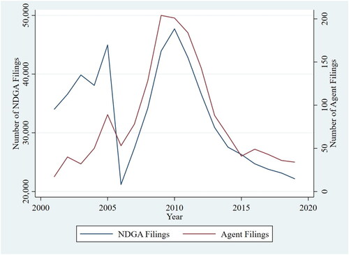
Figure A2. Difference of the housing characteristics before and after matching. Notes: The figure shows the difference of the housing characteristics between two groups of owners, i.e., the previous houses represented by distressed agents versus non-distressed agents, before and after PSM matching.

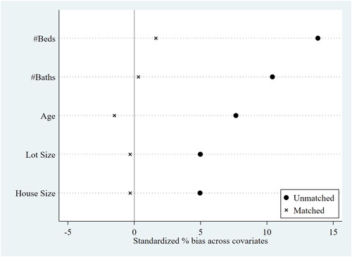
Table A1. Definition of variables.

Variable	Description	Data source
Key variables
Sales price ($)	Transaction price for a property	MLS
if(Distress)	Dummy variable, which indicates whether or not an agent files for the bankruptcy in a given year	Bankruptcy filing
Housing attributes
Baths	The number bathrooms for a given property	MLS
Beds	The number bedrooms for a given property	MLS
Age	The age of a property, which is calculated based on the building year and the listing year.	MLS
House size	Square footage of house size for a given property	MLS
Lot size	Square footage of lot size for a given property	MLS
Others variables
Listing price	Listed price for a property	MLS
TOM (time on market)	how long a property stays on the market before sold	MLS
Pro b(sold)	Whether or not a property is sold eventually	MLS
#Listing	The number of properties listed by an agent each year	Authors’ calculation
#Sales	The number of properties sold by an agent each year	Authors’ calculation
Ratio(#Sales/#Listing)	Ratio of the number of sales over the number of listings for an agent each year	Authors’ calculation
If (downward change)	Whether or not the listing price decreases before the property is sold	Mls
HPI (housing price index)	Housing price index at ZIP code by year level	Zillow Website
If (loan)	Dummy variable, 1 is current home seller takes a loan originated to purchase next house, 0 otherwise	ZTRAX
LTV (loan to value ratio)	Loan to value ratio of next-purchased home	ZTRAX
I (Lower Income)	Dummy variable, 1 is median household income at the new residence (ZIP code) home sellers move to is lower than the previous residence.	Census
I (Lower education)	Dummy variable, 1 is education level (measured by the ratio of Bachelor’s degree) at the new residence (ZIP code) home sellers move to is lower than the previous residence.	Census
I (Lower price)	Dummy variable, 1 is median house price at the new residence (ZIP code) home sellers move to is lower than the previous residence, 0 otherwise	Census

Notes: This table gives the variable names, definition as well as data resources.

Table A2. Additional test of the impact on sale price.

Panel A: Different definitions of treatment periods
	ln(Sales price)
	(1)	(2)	(3)	(4)
if (Distressi,t)	−0.061**	−0.041***	−0.063**	−0.045***
	(−2.34)	(−2.88)	(−2.49)	(−3.33)
Housing attribute	Yes	Yes	Yes	Yes
Agent Individual FE	Yes	Yes	Yes	Yes
Year FE	Yes	No	No	No
Agent location × year FE	No	Yes	No	Yes
Housing market × year FE	No	No	Yes	Yes
N	242,208	242,208	242,208	242,208
R^2	0.771	0.782	0.790	0.799
Panel B: Different thresholds and removing relisted properties
	ln(Sales price)
	(1)	(2)	(3)	(4)
Threshold	2 Transactions	2.5 Transactions	3 Transactions	Remove relisted
if (Distressi,t)	−0.045***	−0.043***	−0.046***	−0.043***
	(−2.58)	(−2.74)	(−2.69)	(−2.65)
housing attribute	Yes	Yes	Yes	Yes
Agent individual FE	Yes	Yes	Yes	Yes
Agent location × year FE	Yes	Yes	Yes	Yes
Housing market × year FE	Yes	Yes	Yes	Yes
N	198,526	150,471	101,124	224,481
R^2	0.732	0.741	0.739	0.789

Notes: Panel A shows the regression results of the impact of personal financial distress on real estate performance when we let if (Distress) (Treatment Period) equal 1 if the listing date or sold date of the house represented by a financially distressed agent is within 6 months before and after the bankruptcy filing month. Panel B presents the regression results when we change the threshold from 1.5 transactions to 2 transactions in Column (1), 2.5 transactions in Column (2), 3 transactions in Column (3) and remove the relisted properties in Column (4). *, **, and *** Denote statistical significance at 10, 5, and 1 percent levels, respectively. Standard errors are clustered at the individual level.

Table A3. Robustness test of impact on sale price.

Panel A: Robustness test on sale price adding controls gradually
	ln(Sales price)
Dep.Var	(1)	(2)	(3)	(4)	(5)	(6)
if (Distressi,t)	−0.034**	−0.023*	−0.024*	−0.025**	−0.021**	−0.040***
	(−2.40)	(−1.84)	(−1.91)	(−2.01)	(−1.99)	(−2.60)
Baths		0.317***	0.234***	0.204***	0.110***	0.105***
		(82.55)	(44.72)	(44.92)	(36.74)	(28.38)
Beds			0.120***	0.109***	0.001	0.001
			(27.01)	(27.44)	(0.54)	(0.28)
Age				−0.013***	−0.010***	−0.011***
				(−69.15)	(−50.57)	(−38.64)
Age^2				0.000***	0.000***	0.000***
				(43.75)	(33.46)	(28.11)
ln(House size)					0.678***	0.641***
					(151.87)	(104.84)
ln(Lot size)						0.065***
						(34.61)
Agent Individual FE	Yes	Yes	Yes	Yes	Yes	Yes
Agent location × year FE	Yes	Yes	Yes	Yes	Yes	Yes
Housing market × year FE	Yes	Yes	Yes	Yes	Yes	Yes
N	448,335	448,335	448,335	434,905	331,636	242,208
R^2	0.561	0.695	0.709	0.727	0.795	0.799
Panel B: Robustness test on sale price using ranges as controls
	ln(Sales price)
Dep.Var	(1)	(2)	(3)	(4)
if (Distressi,t)	−0.042***	−0.024**	−0.044*	−0.023**
	(−2.72)	(–2.06)	(–1.73)	(–2.04)
Baths	0.174***	0.173***	0.164***	0.163***
	(45.86)	(46.29)	(45.15)	(45.50)
Beds	0.051***	0.052***	0.046***	0.047***
	(18.21)	(20.03)	(17.50)	(19.33)
Age	−0.010***	−0.010***	−0.012***	−0.012***
	(–55.49)	(–56.77)	(–65.51)	(–67.17)
Age^2	0.000***	0.000***	0.000***	0.000***
	(38.91)	(39.90)	(43.79)	(45.14)
House size missing	−0.248***	−0.253***	−0.183***	−0.184***
	(–60.20)	(–62.64)	(–37.07)	(–38.16)
House size range 1	−0.515***	−0.512***	−0.503***	−0.502***
	(–117.72)	(–121.59)	(–119.71)	(–123.48)
House size range 2	−0.313***	−0.311***	−0.305***	−0.305***
	(–88.63)	(–90.77)	(–90.14)	(–92.43)
House size range 3	−0.155***	−0.155***	−0.152***	−0.153***
	(–52.25)	(–53.14)	(–53.91)	(–54.89)
Lot size missing	−0.082***	−0.084***	−0.085***	−0.088***
	(–27.91)	(–29.50)	(–29.01)	(–30.90)
Lot size range 1	−0.098***	−0.101***	−0.143***	−0.144***
	(–27.27)	(–29.14)	(–40.83)	(–42.66)
Lot size range 2	−0.081***	−0.081***	−0.108***	−0.108***
	(–25.40)	(–26.49)	(–35.82)	(–36.58)
Lot size range 3	−0.063***	−0.064***	−0.073***	−0.073***
	(–22.40)	(–23.07)	(–27.33)	(–27.75)
Agent individual FE	Yes	Yes	Yes	Yes
Year FE	Yes	No	No	No
Agent location × year FE	No	Yes	No	Yes
Housing market × year FE	No	No	Yes	Yes
N	434,905	434,905	434,905	434,905
R^2	0.735	0.745	0.758	0.766

Notes: This table shows the regression results of the impact of personal financial distress on real estate performance when we add controls gradually, as Panel A shows, and use another specification as control, as Panel B shows. The dependent variable is ln(Sales Price). The independent variable we are interested in is if(Distress). Range 1 means the house size or lot size is below the 25th percentile, Range 2 means the house size or lot size is between the 25th and 50th percentiles, and Range 3 means the house size or lot size is between the 50th and 75th percentiles. The omitted category is house size or lot size is above the 75th percentile. *, **, and *** Denote statistical significance at 10, 5, and 1 percent levels, respectively. Standard errors are clustered at the individual level.

Table A4. Impact of personal financial distress on other outcomes.

Panel A: Impact of personal financial distress on sales probability and volume
	Prob(Sold)	#Listing	#Sales	Ratio(#Sales/#Listing)	#Purchases
Dep. Var	(1)	(2)	(3)	(4)	(5)
if (Distressi,t)	0.004	0.164	0.178	−0.007	0.121
	(0.23)	(0.53)	(0.60)	(−0.65)	(0.65)
Housing attribute	Yes	No	No	No	No
Agent individual FE	Yes	Yes	Yes	Yes	Yes
Agent location × year FE	Yes	Yes	Yes	Yes	Yes
Housing market × year FE	Yes	No	No	No	No
N	437,770	106,452	106,452	106,452	106,452
R^2	0.344	0.342	0.348	0.429	0.347
Panel B: Test of the exit rate after bankruptcy filing
	I(exit)
	(1)
if (Distressi,t)	−0.004
	(−1.31)
Agent individual FE	Yes
Year FE	Yes
N	82,474
R^2	0.011

Notes: Panel A shows the regression results of the impact of personal financial distress on other outcomes, including the probability of sold in Column (1), total the number of listings in Column (2), total the number of sold homes in Column (3), the ratio of the number of sales over the number of listings in Column (4) and total the number of purchased homes in Column (4). The independent variable we are interested in is the dummy variable if(Distress). Note that we use all samples (including both sold and unsold properties) when the dependent variable is Prob(Sold) and use the aggregated agent-year level sample (counted numbers from all samples) when the dependent variable is #Listing, #Sales, Ratio(#Sales/#Listing) and #Purchases. Panel B shows the results of exit rate before and after the bankruptcy filing for distressed vs. non-distressed agents.

References

- Agarwal, S., Ambrose, B. W., & Yao, V. W. (2020). Lender steering in residential mortgage markets. Real Estate Economics, 48(2), 446–475. https://doi.org/10.1111/1540-6229.12203
- Agarwal, S., Amromin, G., Ben-David, I., Chomsisengphet, S., Piskorski, T., & Seru, A. (2017). Policy intervention in debt renegotiation: Evidence from the home affordable modification program. Journal of Political Economy, 125(3), 654–712. https://doi.org/10.1086/691701
- Agarwal, S., Amromin, G., Chomsisengphet, S., Landvoigt, T., Piskorski, T., Seru, A., & Yao, V. (2023). Mortgage refinancing, consumer spending, and competition: Evidence from the home affordable refinance program. The Review of Economic Studies, 90(2), 499–537. https://doi.org/10.1093/restud/rdac039
- Agarwal, S., Amromin, G., Ben-David, I., & Evanoff, D. D. (2016). Loan product steering in mortgage markets (Working paper 22696). https://www.nber.org/papers/w22696.
- Agarwal, S., He, J., Sing, T. F., & Song, C. (2019). Do real estate agents have information advantages in housing markets? Journal of Financial Economics, 134(3), 715–735. https://doi.org/10.1016/j.jfineco.2019.05.008
- Anenberg, E., & Kung, E. (2014). Estimates of the size and source of price declines due to nearby foreclosures. American Economic Review, 104(8), 2527–2551. https://doi.org/10.1257/aer.104.8.2527
- Baker, A. C., Larcker, D. F., & Wang, C. C. (2022). How much should we trust staggered difference-in-differences estimates? Journal of Financial Economics, 144(2), 370–395. https://doi.org/10.1016/j.jfineco.2022.01.004
- Barrot, J. N., & Sauvagnat, J. (2016). Input specificity and the propagation of idiosyncratic shocks in production networks. The Quarterly Journal of Economics, 131(3), 1543–1592. https://doi.org/10.1093/qje/qjw018
- Barwick, P. J., & Pathak, P. A. (2015). The costs of free entry: An empirical study of real estate agents in Greater Boston. The RAND Journal of Economics, 46(1), 103–145. https://doi.org/10.1111/1756-2171.12082
- Barwick, P. J., Pathak, P. A., & Wong, M. (2017). Conflicts of interest and steering in residential brokerage. American Economic Journal: Applied Economics, 9(3), 191–222. https://doi.org/10.1257/app.20160214
- Barwick, P. J., & Wong, M. (2019). Competition in the real estate brokerage industry: A critical review. Brookings Economic Studies. https://www.brookings.edu/wp-content/uploads/2019/12/ES-12.12.19-Barwick-Wong.pdf.
- Bernstein, S., McQuade, T., & Townsend, R. R. (2021). Do household wealth shocks affect performance? Evidence from innovative workers during the great recession. The Journal of Finance, 76(1), 57–111. https://doi.org/10.1111/jofi.12976
- Bian, X., Turnbull, G. K., & Waller, B. D. (2017). Client externality effects of agents selling their own properties. The Journal of Real Estate Finance and Economics, 54, 139–164. https://doi.org/10.1007/s11146-015-9543-y
- Buchak, G., Matvos, G., Piskorski, T., & Seru, A. (2020). Why is intermediating houses so difficult? Evidence from iBuyers (Working paper 28252). https://www.nber.org/papers/w28252
- Callaway, B., Goodman-Bacon, A., & Sant’Anna, P. H. (2021). Difference-in-differences with a continuous treatment (Working paper). https://arxiv.org/abs/2107.02637
- Campbell, J. Y., Giglio, S., & Pathak, P. (2011). Forced sales and house prices. American Economic Review, 101(5), 2108–2131. https://doi.org/10.1257/aer.101.5.2108
- Carvalho, L. S., Meier, S., & Wang, S. W. (2016). Poverty and economic decision-making: Evidence from changes in financial resources at payday. The American Economic Review, 106(2), 260–284. https://doi.org/10.1257/aer.20140481
- Cespedes, J., Liu, Z., & Parra, C. (2020). Almost famous: How wealth shocks impact career choices (Working paper 3491426). https://papers.ssrn.com/sol3/papers.cfm?abstract_id=3491426
- Cunningham, C., Gerardi, K., & Shen, L. (2022). The good, the bad, and the ordinary: Estimating agent value-added using real estate transactions (Working paper 4277192). https://papers.ssrn.com/sol3/papers.cfm?abstract_id=4277192
- Di Falco, S., Berck, P., Bezabih, M., & Köhlin, G. (2019). Rain and impatience: Evidence from rural Ethiopia. Journal of Economic Behavior & Organization, 160(1), 40–51. https://doi.org/10.1016/j.jebo.2019.02.016
- Dimmock, S. G., Gerken, W. C., & Van Alfen, T. (2021). Real estate shocks and financial advisor misconduct. The Journal of Finance, 76(6), 3309–3346. https://doi.org/10.1111/jofi.13067
- Dobbie, W., Goldsmith‐Pinkham, P., Mahoney, N., & Song, J. (2020). Bad credit, no problem? Credit and labor market consequences of bad credit reports. The Journal of Finance, 75(5), 2377–2419. https://doi.org/10.1111/jofi.12954
- Geltner, D., Kluger, B. D., & Miller, N. G. (1991). Optimal price and selling effort from the perspectives of the broker and seller. Real Estate Economics, 19(1), 1–24. https://doi.org/10.1111/1540-6229.00537
- Gerardi, K., Rosenblatt, E., Willen, P. S., & Yao, V. (2015). Foreclosure externalities: New evidence. Journal of Urban Economics, 87(1), 42–56. https://doi.org/10.1016/j.jue.2015.02.004
- Giroud, X., & Mueller, H. M. (2019). Firms’ internal networks and local economic shocks. American Economic Review, 109(10), 3617–3649. https://doi.org/10.1257/aer.20170346
- Gilbukh, S., & Goldsmith-Pinkham, P. (2023). Heterogeneous real estate agents and the housing cycle (Working paper 31683). https://www.nber.org/papers/w31683
- Goette, L., Huffman, D., & Fehr, E. (2004). Loss aversion and labor supply. Journal of the European Economic Association, 2(2–3), 216–228. https://doi.org/10.1162/154247604323067934
- Goodman-Bacon, A. (2021). Difference-in-differences with variation in treatment timing. Journal of Econometrics, 225(2), 254–277. https://doi.org/10.1016/j.jeconom.2021.03.014
- Guiso, L., Pozzi, A., Tsoy, A., Gambacorta, L., & Mistrulli, P. E. (2022). The cost of steering in financial markets: Evidence from the mortgage market. Journal of Financial Economics, 143(3), 1209–1226. https://doi.org/10.1016/j.jfineco.2021.05.013
- Han, L., & Hong, S. H. (2011). Testing cost inefficiency under free entry in the real estate brokerage industry. Journal of Business & Economic Statistics, 29(4), 564–578. https://doi.org/10.1198/jbes.2011.08314
- Han, L., & Hong, S. H. (2016). Understanding in‐house transactions in the real estate brokerage industry. The Rand Journal of Economics, 47(4), 1057–1086. https://doi.org/10.1111/1756-2171.12163
- Harding, J. P., Rosenblatt, E., & Yao, V. W. (2009). The contagion effect of foreclosed properties. Journal of Urban Economics, 66(3), 164–178. https://doi.org/10.1016/j.jue.2009.07.003
- Heckman, J. J. (1979). Sample selection bias as a specification error. Econometrica, 47(1), 153–161. https://doi.org/10.2307/1912352
- Hsieh, C. T., & Moretti, E. (2003). Can free entry be inefficient? Fixed commissions and social waste in the real estate industry. Journal of Political Economy, 111(5), 1076–1122. https://doi.org/10.1086/376953
- Johnson, K. H., Lin, Z., & Xie, J. (2015). Dual agent distortions in real estate transactions. Real Estate Economics, 43(2), 507–536. https://doi.org/10.1111/1540-6229.12073
- Kaur, S., Mullainathan, S., Oh, S., & Schilbach, F. (2021). Do financial concerns make workers less productive? (Working paper 28338). https://www.nber.org/papers/w28338
- Khwaja, A. I., & Mian, A. (2008). Tracing the impact of bank liquidity shocks: Evidence from an emerging market. American Economic Review, 98(4), 1413–1442. https://doi.org/10.1257/aer.98.4.1413
- Levitt, S. D., & Dubner, S. J. (2014). Freakonomics. HarperCollins (ISBN:9780141019017).
- Levitt, S. D., & Syverson, C. (2008). Market distortions when agents are better informed: The value of information in real estate transactions. Review of Economics and Statistics, 90(4), 599–611. https://doi.org/10.1162/rest.90.4.599
- Levitt, S. D., Syverson, C., & Ferreira, F. (2008). Antitrust implications of outcomes when home sellers use flat-fee real estate agents. Brookings-Wharton Papers on Urban Affairs, 2008, 47–93. https://doi.org/10.1353/urb.2008.a249797
- Lin, Z., Liu, Y., & Xie, J. (2024). Market distortions with collusion of agents. Journal of Banking & Finance, 162, Article 107151. https://doi.org/10.1016/j.jbankfin.2024.107151
- Lopez, L. A., McCoy, S. J., & Sah, V. (2022). Steering consumers to lenders in residential real estate markets. Real Estate Economics, 50(6), 1596–1641. https://doi.org/10.1111/1540-6229.12386
- Maggio, M. D., Kalda, A., & Yao, V. (2019). Second chance: Life without student debt (Working paper 25810). https://www.nber.org/papers/w25810
- Mast, B. D., & Din, A. (2021). Measuring neighborhood opportunity with opportunity atlas and child opportunity index 2.0 data. Cityscape, 23(1), 237–256. https://www.jstor.org/stable/26999947
- Maturana, G., & Nickerson, J. (2020). Real effects of workers’ financial distress: Evidence from teacher spillovers. Journal of Financial Economics, 136(1), 137–151. https://doi.org/10.1016/j.jfineco.2019.09.001
- Mian, A., Sufi, A., & Trebbi, F. (2015). Foreclosures, house prices, and the real economy. The Journal of Finance, 70(6), 2587–2634. https://doi.org/10.1111/jofi.12310
- Moulton, S., Chun, Y., Casey Pierce, S., Quercia, R., Riley, S., & Holtzen, H. (2022). Does temporary mortgage assistance for unemployed homeowners reduce longer‐term mortgage default? An analysis of the hardest hit fund program. Journal of Policy Analysis and Management, 41(2), 515–551. https://doi.org/10.1002/pam.22346
- Pool, V. K., Stoffman, N., Yonker, S. E., & Zhang, H. (2019). Do shocks to personal wealth affect risk-taking in delegated portfolios? The Review of Financial Studies, 32(4), 1457–1493. https://doi.org/10.1093/rfs/hhy096
- Rizzo, J. A., & Zeckhauser, R. J. (2003). Reference incomes, loss aversion, and physician behavior. Review of Economics and Statistics, 85(4), 909–922. https://doi.org/10.1162/003465303772815817
- Robles-Garcia, C. (2019). Competition and incentives in mortgage markets: The role of brokers (working paper). Stanford Business.
- Rutherford, R. C., Springer, T. M., & Yavas, A. (2005). Conflicts between principals and agents: Evidence from residential brokerage. Journal of Financial Economics, 76(3), 627–665. https://doi.org/10.1016/j.jfineco.2004.06.006
- Rutherford, R., & Yavas, A. (2012). Discount brokerage in residential real estate markets. Real Estate Economics, 40(3), 508–535. https://doi.org/10.1111/j.1540-6229.2011.00319.x
- Smith, P. S., Gibler, K. M., & Zahirovic-Herbert, V. (2016). The effect of relisting on house selling price. The Journal of Real Estate Finance and Economics, 52, 176–195. https://doi.org/10.1007/s11146-015-9503-6
- Tanaka, T., Camerer, C. F., & Nguyen, Q. (2010). Risk and time preferences: Linking experimental and household survey data from Vietnam. American Economic Review, 100(1), 557–571. https://doi.org/10.1257/aer.100.1.557
- Turnbull, G. K., Waller, B. D., & Wentland, S. A. (2022). Mitigating agency costs in the housing market. Real Estate Economics, 50(3), 829–861. https://doi.org/10.1111/1540-6229.12349
- Townsend, R. R. (2015). Propagation of financial shocks: The case of venture capital. Management Science, 61(11), 2782–2802. https://doi.org/10.1287/mnsc.2014.2110
- Weisbach, M. S. (1988). Outside directors and CEO turnover. Journal of Financial Economics, 20(1), 431–460. https://doi.org/10.1016/0304-405X(88)90053-0
- Yavas, A. (2007). Introduction: Real estate brokerage. The Journal of Real Estate Finance and Economics, 35(1), 1–5. https://doi.org/10.1007/s11146-007-9030-1
- Zahirovic-Herbert, V., & Gibler, K. M. (2014). Historic district influence on house prices and marketing duration. The Journal of Real Estate Finance and Economics, 48, 112–131. https://doi.org/10.1007/s11146-012-9380-1