Simulation-driven design of a fast monohull

ABSTRACT

A fast monohull was designed and optimized, using CAESES® for parametric modeling and optimization coupled to STAR-CCM + for free-surface RANS simulations. The boat is a 9.5ton pilot boat, featuring tunneled propellers, shafts and rudders. The optimizations were undertaken for thrust at design speed of 27.5kn. The boat was free to trim and rise, utilizing an overset grid for high resolution and acceptable turn-around time. Propulsion was taken into account via an actuator disc, balancing resistance and thrust. The geometry of the bare hull and tunnel were varied during the optimizations, using fully-parametric models. A systematic comparison of numerical and experimental data was undertaken. The experiments were conducted with the high-speed carriage at TU Berlin, using a 3.5m fully-appended self-propelled model. The optimizations comprised Design-of-Experiments, deterministic searches, surrogates and global strategies. Substantial improvements were found with variants being more energy-efficient than a representative baseline. The paper discusses modeling, simulations and optimizations along with selected results.

KEYWORDS:

• Simulation-driven Design (SDD)
• parametric modeling
• formal optimization
• Computational Fluid Dynamics (CFD)
• Computer Aided Engineering (CAE)
• planing boat
• Design-Of-Experiment (DoE)
• machine learning (ML)

1. Introduction

1.1. Historical context

‘To optimize is human.’ This was the opening statement by Horst Nowacki (2003) in his contribution to the 39th WEGEMT school (Birk and Harries 2003). Being aware of a need, deliberately searching for an optimum, considering the constraints and intending to use the freedom available in a given situation may well be one of the defining characteristics of mankind. Very likely, optimization has always been a human trait and it will always be – maybe even more so with eight billion human beings on planet Earth, officially declared on November 15, 2022. Looking at our extraordinary consumption of resources, sustainability can only be achieved if we all strive to produce and use energy as efficiently as possible.

In engineering, the approach of formal optimization has been researched and developed since the middle of the twentieth century, picking up momentum with the increase of computational resources. In naval architecture and in ship hydrodynamics in particular, numerical optimizations date back to the 1960s, for instance, Lin et al. (1963) as well as Pien and Moore (1963). Being able to compute the flow about a body by means of potential flow theory as independently introduced by Hess and Smith (1962) and Nowacki (1963) and, subsequently, to approximate the wave resistance of ships for the actual hull form, giving an understanding of cause-and-effect of geometry and flow field, inspired both academia and industry. For a review see Harries (1998), covering publications up to the late 1990s, and Harries (2020) for a summary of some more recent contributions.

Over the last decades, consequently, many fields of science – in particular, geometric modeling, flow simulation and optimization methods – have been expanded and suitably combined in order to undertake what is presently called simulation-driven design (SDD), see Harries and Abt (2019a) as well as Harries (2020). The term reflects that simulations are utilized extensively to identify designs that are optimal or, at least, superior to a known solution, often referred to as the baseline. This implies that not only a handful of manually created options are examined with the help of simulations – a process commonly termed simulation-based design (SBD) – but that a large number of designs – digital siblings, so to speak, see Papanikolaou (2024) – are generated automatically by and during the process.

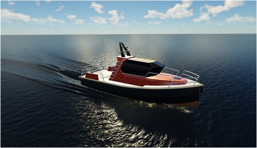
This paper presents the simulation-driven design of a fast monohull at a design speed of 27.5kn. The boat is about 11 m in length and 3.5 m in beam with a displacement of 9.5ton at a design draft of 0.6 m, see also Table 4. It shall serve as a pilot boat and is built by UZMAR in Turkey. Figure 1 gives an artist’s impression, showing the actual wave field from the numerical simulations.

Figure 1. Illustration of the planing boat in calm water. (SkyView in CAESES with wave field from Simcenter STAR-CCM+).

1.2. R&D project AutoPlan

The work was undertaken within the European R&D project AutoPlan under the umbrella of the MarTERA program with the primary goal of gaining a better understanding of the hydrodynamics of planing boats by investigating them numerically as well as physically at both model- and full-scale.

In the first stage of the project, a fully parametric model is developed by FRIENDSHIP SYSTEMS, Germany, using CAESES® based on a preliminary design provided by the Turkish shipyard and project leader UZMAR. From this a first and a new baseline plus an optimized design are thoroughly studied numerically and, subsequently, investigated experimentally at Technical University Berlin’s section of Dynamics of Maritime Systems.

One of the key tasks of AutoPlan is a comprehensive performance optimization of the planing hull – which is presented in detail in this paper. This requires extensive numerical simulations and suitable validations by means of model tests. The tests are undertaken in TU Berlin’s 250 m long towing tank (formerly known as VWS) with fully equipped scale models at a model scale of 3.2871. The models are produced by SVA Potsdam, Germany. The baseline features an exchangeable tunnel section for preliminary studies and validation. From the optimization campaigns, as discussed here, the final design is chosen by UZMAR, taking into account practical aspects and the operational profile as a pilot boat.

In addition, a mathematical model to predict the maneuvering of the planing boat is developed at TU Berlin. This forms another key task of the AutoPlan project, namely, the development of a better understanding of possible instabilities like porpoising which planing boats occasionally encounter and whose inceptions are difficult to predict. The results of this project stage are validated by means of experiments at both model- and full-scale.

The maneuvering models are used by OES, Turkey, to build a system, the so-called Intelligent Navigation System (INA), to support the boat’s crew in avoiding potentially harmful situations. At the final stage of the project the operation of the various models and systems along with the power prediction are to be tested onboard a full-scale prototype built in aluminium by UZMAR and equipped with a thrust gauge developed by SVA. Photos taken during the sea trials are presented in Appendix I for illustration.

1.3. Planing

The definition of when a boat is already planing is somewhat ambiguous. Typical criteria are that a considerable portion of weight is supported by hydrodynamic lift, that the centre of gravity rises (negative sinkage), that trim is positive (bow up) and that the transom is fully ventilated. As shown in this paper these criteria are all fulfilled.

Based on the main dimensions at the design speed of 27.5kn the Froude number based on length (at rest) is Fn = 1.36 while the Froude numbers computed with displacement and beam at the transom are FnV = 3.12 and FnB = 2.41, respectively. The latter number is also known as the speed coefficient used by Savitsky and Brown (1976). It is already quite high, again suggesting planing mode.

Nevertheless, a formal partitioning of regimes is also done by means of the volumetric Froude number where F_n∇ < 1.5 characterizes displacement ships, 1.5 < F_n∇ < 3 indicates semi-displacement or semi-planing vessels and 3 < F_n∇ is typical of planing boats. Therefore, it should be kept in mind that at design speed the pilot boat presented here is at the lower end of planing.¹

1.4. Outline

This paper is organized as follows: On the basis of the brief introduction of simulation-driven design and the background of the AutoPlan project, see above, the parametric models for the bare hull and the tunnel, respectively, along with the assembly of the geometry and the possibility of automated form variations are explained in section 2. This is followed by a discussion about the CFD set-up in section 3 where focus is put on fast yet accurate simulations. An encouraging comparison is included between CFD results and measurements from model tests. Section 4 then presents manual improvements and, setting out from them, the simulation-driven design campaigns and their most important results. Section 5 gives a brief outlook while section 6 summarizes the main conclusions.

Since the paper is rather comprehensive a commented outline is given in Table 1. Complementing each section, additional pieces of information are given in corresponding appendices.

Table 1. Outline of the paper.

	Section	Content	Purpose
1.	Introduction	• Historical background and motivation • R&D project AutoPlan	Set the context of the paper as part of the special issue in honour of late Prof. Dr.-Ing. Dr. h.c. Horst Nowacki
2.	Parametric model	• Parametric model of the bare hull • Parametric model of the tunnel • Assembly and variation of bare hull and tunnel	Present the modeling approach and the chosen form parameters for SDD
3.	CFD simulations	• Thrust as objective • Computational set-up • Grid convergence and uncertainty • Comparison between CFD and EFD	Explain how the objective is computed efficiently with reasonable accuracy
4.	Simulation-driven design	• Manual improvements • SDD campaigns - Exploration (DoE) - Exploitation (deterministic search) - Surrogate • Flow fields and geometry of selected designs	Discuss how a competitive baseline is realized, following a simulation-based design approach; present the various SDD campaigns and results
5.	Off-design conditions and outlook	• Performance at different speeds and displacements • Further model tests and full-scale prototype • Additional methods of SDD	Show robustness of optimum; give an appreciation of further experimental work within AutoPlan; put work presented into context with additional methods
6.	Conclusions	• Main conclusions as derived from the various sections and results	Summarize findings

2. Parametric model

2.1. Approach

When optimizing a product the effort of exploring the design space and of exploiting the potential of further improvement scales up rapidly with the number of free variables of the systems, i.e. the degree-of-freedom (DoF). The more free variables the more variants are needed, Harries (2020). Consequently, instead of allowing any conceivable freedom a deliberate reduction of variability is built into a system. Usually, this is realized by defining a product with as few descriptors, typically called parameters, as possible. In Computer Aided Design (CAD) this approach is generally referred to as parametric modeling.²

For the planing boat a fully parametric approach was taken since it allows high flexibility along with very detailed control. Firstly, a bare hull was defined based on the specifications from the yard and considering recommendations given by Larsson et al. (2014), Savitsky and Brown (1976) and Savitsky (1964). Secondly, a tunnel was modelled so as to accommodate the propellers, shaft lines, brackets and rudders as designed and provided by an external supplier. Subsequently, the bare hull and the tunnel were combined and complemented by a headbox for a smooth transition to the rudder.

2.2. Bare hull

The fully parametric modeling of the bare hull follows the approach introduced by Harries (1998) and builds on the model developed for the simulation-driven design of a fast monohull presented by Albert et al. (2016).³

It uses a specialized surface object called MetaSurface, a dedicated sweep surface provided in CAESES®. It allows combining a parameter-based shape definition in one direction, i.e. a user-specified pattern (called curveEngine in CAESES), with user-specified basic curves that run into another direction, usually somewhat perpendicular to the first. The basic curves supply the values for all parameters that are needed to generate the geometry at any given position along the sweep. The final outcome is a parametrically defined B-spline surface whose vertices are fully determined from both the pattern and the basic curves without any manual positioning in space. For further details see Harries et al. (2015) as well as Albert et al. (2016).

Figures 2–5(A) presents the basic curves in side view (projection in y-direction), top view (projection in z-direction), front view (projection in x-direction) and perspective view, respectively, along with the resulting surfaces. The two surfaces that are most relevant to the planing of the hull are the bottom and the spray rail. The bottom is a MetaSurface that runs from the keel line and stem contour (modelled as a polyCurve) to a 3d-curve for the inner spray rail (modelled as a genericCurve made up from projections in y- and z-direction). The spray rail itself is a simple ruledSurface, spanning from the curves for the inner to the outer spray rails, respectively. Similar to the curve for the inner spray rail the curve for the outer spray rail is made up from two projections. This allows defining parameters conveniently in both the x-y-plane and the x-z-plane.

Figure 2. Side view of bare hull without tunnels.

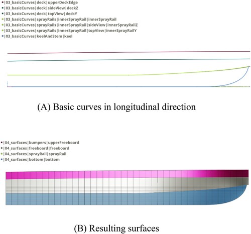
Figure 3. Top view of definition of bare hull without tunnels.

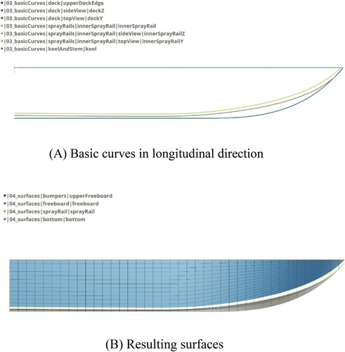
Figure 4. Front view of bare hull without tunnels.

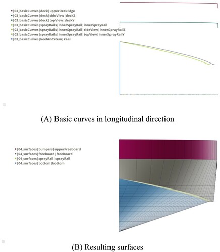
Figure 5. Perspective view of bare hull without tunnels.

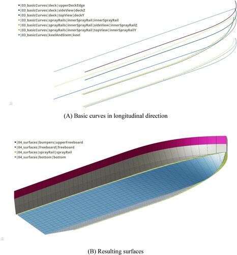
The freeboard and the upper part of the boat’s side (bumper) are also defined as ruledSurfaces, the deck again being modelled via projections. When the boat is planing these surfaces typically are dry since the water detaches at the outer edge of the spray rail.

Figures 2(B)–5(B) show the bottom in blue, the spray rail in green, the freeboard in grey and the bumper in red. For a closed definition of the entire hull a transom (as several ruledSurface) and a deck (as a MetaSurface) are added (not shown here).

All basic curves are defined via parameters that give positions, angles or integral values, see Harries (1998). Tables 2 and 3 summarize global and local parameters for the bare hull, respectively. By changing any of the parameters all entities within the model are successively updated, resulting in a new geometry, see Harries and Abt (2019b) for an elaboration on hierarchy and client-supplier relationships. For variations of the bare hull see Appendix II.

Table 2. Global parameters of the planing boat (parameters featuring sliders are free variables with given lower and upper bounds).

Table 3. Parameters of basic curves.

For the simulation-driven design campaign the length of the boat and the beam were kept constant, following a request by the shipyard. It should be noted that, in general, any parameter within a model could potentially be used as a free variable, provided it does not have any suppliers, i.e. it does not depend on other parameters, see Harries and Abt (2019b). Here a subset of parameters as shown in Tables 2 and 3 is used within the various campaigns, complemented by parameters for the tunnel as shown in Table 4.

Table 4. Parameters of the tunnel (N.B. The tunnel radius is kept constant during the optimizations).

2.3. Tunnel

The shipyard opted for a conventional propulsion package with two engines, straight shafts, I-brackets and spate rudders. In order to decrease the planing boat’s overall draft and to realize a small inclination angle of the shaft lines, the propellers are placed inside elongated tunnels. Design guidelines by Blount (2023) were taken into consideration, subdividing each tunnel into an entrance region, a propeller region and an exit. The tunnel radius at the longitudinal position of the propeller is chosen to give sufficient clearance, the tunnel’s circular segment above the propeller being concentric to the propeller’s centre.

Table 4 gives an impression of the parameters that define the tunnel: The entrance region smoothly takes off from the bare hull and curves upward to the maximum tunnel clearance. The propeller region essentially is parallel with flexible start and end positions forward and aft of the propeller’s centre, respectively. The exit allows for both a flattening and a sideways ‘squeeze’ of the round opening at the transom along with a downward inclination of the top contour so as to introduce an integrated wedge. This is motivated by the wish to.

• Reduce potential air intake when going backward,

• Encapsulate the headbox for the rudder smoothly,

• Introduce additional lift to help raise the transom upward, and,

• Direct the accelerated flow from the propeller aft of the transom.

The tip of the tunnel where it transits into the bare hull is free to move forward and backward while, in addition, it can be shifted inward and outward to align it with the local streamlines.

The geometry of the tunnel was modelled by means of a so-called Gordon surface that takes a mesh of longitudinal and transversal curves as input, see also Albert et al. (2021). Figure 6 depicts the entities that define the tunnel in perspective view. Figure 6(A) shows the inner and outer rails of the tunnel along with the tunnel’s top contour. Figure 6(B) gives the transversal curves. Each of them is an arc derived from three associated points lying on the rails and the top contour, respectively. Figure 6(C) shows the resulting surface that takes all nine transversal curves plus the two rails as longitudinal curves as input, yielding a smoothly interpolating surface as illustrated via isophotes in Figure 7. The top contour is captured discretely via the transversal curves that interpolate it.

Figure 6. Tunnel geometry defined via a Gordon surface.

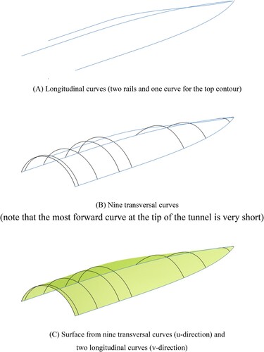
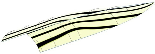
Figure 7. Isophotes on tunnel modelled as a Gordon surface.

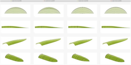
Varying the tunnel parameters, e.g. by means of a DoE, yields distinctively different shapes. Four representative tunnels are shown in Figure 8 via a screen shot from CAESES’ DesignViewer. The form parameters, should be understood, control the rails and the top contour. Meanwhile, the transversal curves are determined from the longitudinal curves. The Gordon surface, finally, interpolates the transversal curves and, consequently, is fully defined by means of the parameters without any need for any interactivity.

Figure 8. Example variations of the tunnel (before assembly with the bare hull).

2.4. Assembly

The bare hull and the tunnel being established as BReps (boundary representations), they need to be assembled to yield the final shape of the tunneled hull. BReps are trimmed NURBS surfaces which form the basis of solid modeling of complex shapes via Boolean operations. Here, the tunneled hull is realized by means of subtracting the tunnel from the bare hull as indicated in Figure 9.

Figure 9. Perspective view of assembly of final hull from bare hull and tunnel. (A) Tunnel geometry (green surface) converted into a solid and rotated to position (grey), protruding into the bare hull (semi-transparent solid in blue for the bottom and the freeboard with purple for the transom); (B) Imprint of the tunnel (green region) in solid for the bare hull (blue).

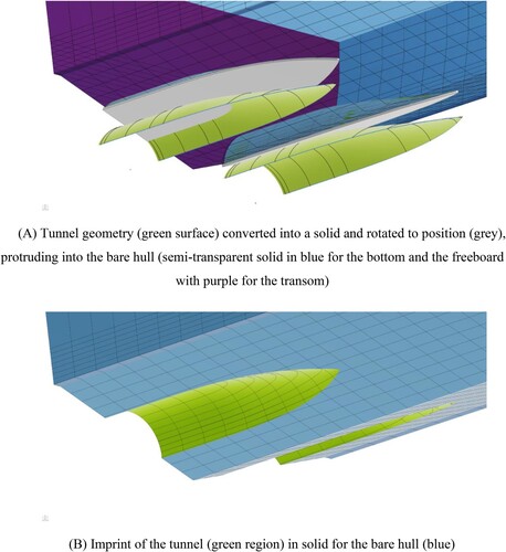
The tunnel surface, modelled as described above, is slightly extruded downstream (in negative x-direction) and downward (in negative z-direction) for robustness to avoid having to intersect coplanar objects. It is then converted into a solid and subsequently rotated to the correct position above the propeller, Figure 9(A). Following the Boolean operation, the tunnel shows up as an imprint to the bare hull, creating a complex but watertight tunneled hull, Figure 9(B).

Figure 10 gives an impression of the aftbody with all components put together. (Note that the shaft line and the bracket were approximated for the sake of illustration in order to protect the IPR of the supplier. For the same reason the propeller does not represent the final design either.) The propeller position is shown as a turquoise disc so that the concentricity of the propeller, before being rotated to align with the shaft, and the tunnel becomes apparent.

Figure 10. Perspective view of aftbody with all components put together (shaft line and bracket conceptually approximated for illustration).

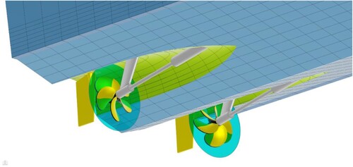
The assembly of the bare hull and the tunnel features sharp edges. In principle, a round transition could be modelled, too, if this was the preference of the designer. Figure AII.2 offers a stern view of the fully appended boat.

Finally, it should be pointed out that the rudder, also provided by a supplier, is connected to the tunnel via a headbox. The headbox is parametrically defined, too, but is quite small and is not actively modified during the optimization campaigns. It simply adjusts to variations of the tunnel. Moreover, the rudder was left out of the CFD analyses during the optimization as a sacrifice to save some computational resources. Therefore, neither the headbox nor the rudder shall be further discussed here for reasons of space.

2.5. Variation of the fully appended hull

The parametric model realized in CAESES® allows selecting any parameter that does not depend on any other parameter or expression. Consequently, for optimization campaigns the design team can choose to vary the bare hull only, keeping the tunnel geometry constant, vary the tunnel for any given bare hull or vary both bare hull and tunnel at the same time.

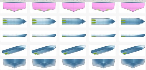
Figure 11 depicts example variations of the hull for a given tunnel. See also Figure AII.1 for variations of the bare hull without tunnel for comparison.

Figure 11. Example variations of the bare hull with tunnel.

3. CFD simulations

3.1. Choice of the objective

In order to quantify the performance of different variants that can be created either manually by a designer or automatically by means of an algorithm, using parametric modeling as explained above, RANS simulations are performed, taking into account viscosity, the free surface, dynamic trim and rise of the vessel, and the effect of the propulsor. The simulations are run in Simcenter STAR-CCM+, a versatile Computational Fluid Dynamics code (CFD) known for its accuracy. This section describes the chosen CFD set-up along with the selection of an appropriate objective for the optimizations.

The right choice of objective(s) is essential for any optimization task and depends on the preferences of the future owner or operator. For the optimization of displacement hulls resistance has often been used to compare designs via both tank tests and CFD. Horizontal forces are measured and the resistance is ranked. In the last decade, more often power delivered has been targeted, giving a more comprehensive picture. This is also the direction to take for high-speed boats.

Semi-planing and planing hulls are often relatively light and run at tangible trim angles and are partially raised out of the water when going fast, the weight of the vessel then being partially supported by dynamic lift. The presence of a propeller directly influences the swimming conditions and the wetted surface area differs significantly from the situation at rest. Therefore, in the context of optimizing planing hulls for either minimum energy consumption or maximum speed it is of importance to take propulsion into account.

Here, total thrust is used as a single objective, using the open water curves of the propeller provided by the shipyard’s supplier of the propulsion unit. Instead of representing the true geometry of the propeller at the revolutions needed to achieve design speed, the propeller was modelled by means of a so-called body force propeller method as made available in Simcenter STAR-CCM +. The former would be possible, in principle, but would take even more computational resources.

Figure 12 shows the appended hull exported from CAESES via a STEP-file and imported into STAR-CCM +. It can be seen that the propeller is substituted by an actuator disc. The shafts and brackets are considered, too, as they influence the pressure distribution and the wake field. However, the rudders are neglected for the optimizations, again in order to save resources as mentioned already. Finally, it needs to be noted that all CFD analyses are run at model-scale for direct comparison to experimental data. Further details are given in Ahmed (2022).

Figure 12. Appended hull with actuator disk for CFD simulations within Simcenter STAR-CCM + (rudder omitted).

3.2. Principal dimensions and definitions

The boat’s principal dimensions are summarized in Table 5. The coordinate system is placed at the transom where the aft perpendicular (AP) is formally located. The x-direction points forward to the bow. The coordinate system’s origin lies at the bottom and in the symmetry plane, the z-direction going upward and the y-direction pointing towards the portside.

Table 5. Principal dimensions at full-scale and at model scale (model scale of 3.2871).

Parameter	Symbol	Full-scale	Model-scale	Units
Length over all	LOA	11.058	3.364	m
Beam	B	3.5	1.065	m
Design displacement	Δ	9.5	0.267	ton
Draft	D	0.611	0.186	m
Longitudinal centre of gravity from AP	LCG	4.945	1.504	m
Vertical centre of gravity from base	VCG	0.7	0.213	m
Design speed	V	27.5	15.168	kn
Froude number	Fn	1.358	1.358	–
Attachment point of towing force in longitudinal direction from AP	TPX	5.529	1.682	m
Attachment point of towing force in vertical direction from AP	TPz	0.611	0.186	m

The position of both the centre of gravity (CoG) and the towing point (TP) for drag reduction excited during the model tests are measured from the origin of the coordinate system, see Table 5. The boat’s heave (i.e. negative sinkage) and trim (pitch) are given at the CoG. A positive value of heave corresponds to a rise in the upward direction while a positive trim angle, by convention, represents bow up. As the simulations are undertaken to reflect the towing tank set-up the same towing point is used in both the experiments and the simulations, given by TP_X and TP_Z in Table 5 where TP_Y = 0.

Resistance (drag) which is used for grid convergence and validation studies represents the horizontal force experienced by the vessel moving forward. Propeller thrust as the objective for the optimization is always measured in the propeller plane along the engine shaft line which is inclined at an angle of 10 degrees measured from the keel line at rest. All of these conventions are kept consistent throughout the studies to allow meaningful comparisons.

3.3. Discretization approach and computational set-up

Simulating marine applications with RANS codes requires appropriate mesh discretization strategies. The International Towing Tank Conference (ITTC) has documented guidelines for various types of vessels, ITTC (2014).

Simulating high Reynolds number requires very fine discretization in both temporal and spatial domains. This scales up substantially with larger changes of the swimming condition for fast boats. Performing optimizations by simulating dozens or even hundreds of variants with very fine meshes is rather expensive. In addition, large changes in running attitude may result in mesh distortion and numerical ventilation as explained in Wheeler et al. (2021). To handle this situation accurately and efficiently, a dynamic overset grid is used in combination with an adaptive mesh refinement for both the overset and the free surface region, complemented by a volume-of-fluid (VOF) slip velocity method, see Wheeler et al. (2021). Figure 13. illustrates the domain around the hull in which an overset grid⁴ is utilized.

Figure 13. Overset grid around the ship within Simcenter STAR-CCM +.

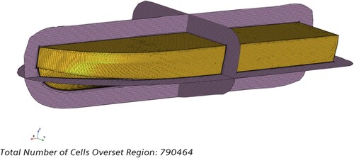
For an overset grid (at least) two different meshes, known as background and overset mesh, respectively, are combined. The background mesh is typically used for the major part of the fluid domain that does not change. In the background mesh the cells lying within the overset mesh are inactive. The overset mesh is usually built for a smaller part of the domain and wraps around the object that supposedly changes position during the simulation. The primary advantage is to avoid excessive mesh distortion for large displacements of that object, here the considerable changes in running attitude of the hull. This means that the overset mesh around the hull moves with trim and rise and, by keeping the mesh geometry undistorted, its quality is maintained, e.g. in terms of y ⁺-values in the boundary layer.

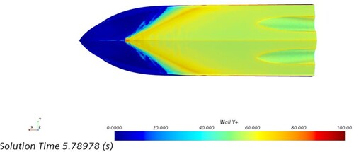
In the STAR-CMM + set-up for the fast monohull the overset domain uses prism layers near the walls and a structured mesh otherwise. The prism layer thickness is adapted to have wall y ⁺-values of around 70, making it possible to apply the realizable k-epsilon turbulence model with wall functions. Figure 14 shows the distribution of y⁺ on the hull at the final step of the solution.

Figure 14. y⁺ distribution on the hull at convergence (bottom view) within Simcenter STAR-CCM +.

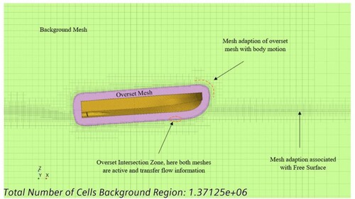
The information transfer between the background mesh and the overset mesh is done with the so-called overset algorithm. This requires a transitional domain of similar cell sizes called mesh intersection zone. This zone features a few cells from both meshes that overlap to ensure proper exchange of data. Figure 15 illustrates the overset grid in combination with free surface adaptive mesh refinement. Additional illustrations are given in Appendix II.

Figure 15. Overset grid with adaptive mesh refinement.

3.4. Numerical set-up

In order to be able to run many variants of this high-speed vessel, a numerical set-up needs to be chosen that is fast yet still reasonably accurate. While the mesh discretization and the use of an overset grid are discussed in the previous section, the physical set-up along with the boundary conditions are presented below. The main settings are as follows:

• Symmetry is applied along the centreline of the hull and only half of the domain is meshed and simulated.

• A segregated fluid solver for incompressible fluids is used.

• A semi-implicit pressure linked equations scheme (SIMPLE) is employed.

• During the transient acceleration phase while increasing speed, a first-order pseudo state transient solver is applied in order to reach steady state operating conditions quickly. (This means that the flow fields computed at intermediate steps do not represent physics meaningfully. Initially, the free surface is not refined either.)

• A Reynolds-Averaged-Navier-Stokes (RANS) based realizable k-epsilon model with wall function approach is employed to account for turbulence.

• A volume-of-fluid (VOF) scheme to capture the free surface using a high resolution interface capturing scheme (HRIC) is employed.

A difference in computing high-speed vessels – compared to displacement ships – is the large change of running attitude caused by the hydrodynamic forces acting on the hull which can either be computed by solving the motion equations in every time step or by successively computing multiple steady-state simulations, adjusting rise and trim iteratively. In the present application, the first method is chosen. To improve convergence, a smooth ramp-up of the velocity is used. The three DoF (prescribed surge, computed heave and trim) are considered for the overset region, while the background domain follows the overset region in longitudinal direction (1 DoF).

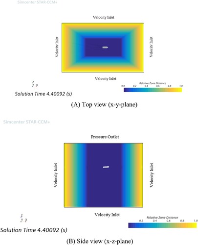
The imposed translation of the background mesh uses wave forcing treatment, applied near the vertical wall region called buffer layer as shown in Figure 16(A) and (B). Velocity inlets with zero velocity are prescribed at the domain boundaries, while a pressure boundary condition at the top of the domain ensures a hydrostatic gradient. Near the vessel boundaries and in the overset region, no-slip boundary conditions are imposed. Symmetry conditions along the centre plane are employed to reduce computational time. Wave forcing is achieved by applying an additional term on the right hand side of the momentum equations during the numerical simulations. Further elaborations are given in Appendix III.

Figure 16. Wave forcing zones and boundary conditions (bow pointing to the right).

3.5. Grid convergence

In order to identify a mesh that yields accurate results fast enough for optimization systematic grid convergence studies are undertaken with mesh sizes from 0.4 million to 5.7 million cells. The meshes in the background and the overset regions are varied via a ‘refinement ratio’ R as defined by Xing and Stern (2010). It defines changes in mesh sizes and ensures that the ratio of cells present in the background and in the overset region is maintained and, hence, that the cell sizes in the intersection zone match.

Background and overset meshes are varied according to L_PP/(5 R) and L_PP/(100 R), respectively. Here L_PP is the length between perpendiculars at model-scale with 3.364 m. R values start from ½ and increase by a factor of √2 with finer grid sizes. Table 6 summarizes the mesh sizes along with results for drag (total resistance), heave (rise) and pitch (trim).

Table 6. Grid convergence study.

	Base Size
Name	Back-ground	Overset	Total # of cells	Time	Refinement ratio R	Heave	Pitch	Drag
	m	m		hours		cm	deg	N
Mesh 1	1.35	0.065	408 676	1.22	1 / 2	10.58	4.987	526.36
Mesh 2	0.95	0.050	831 152	2.21	√2 / 2	10.73	5.105	569.42
Mesh 3	0.67	0.035	1 755 600	3.79	1	10.49	5.004	535.57
Mesh 4	0.48	0.025	3 661 000	5.20	√2	10.67	5.100	520.56
Mesh 5	0.40	0.020	5 745 000	10.2	2	10.68	5.143	519.27

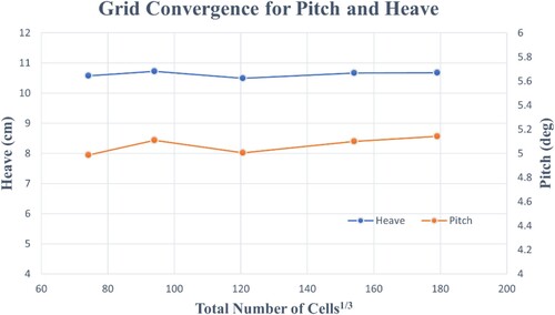
To monitor convergence with varying grids the values of drag, heave and pitch are plotted vs. the total number of cells, see Figures 17 and 18. Apparently, drag converges after Mesh 3 since results are very similar for Meshes 4 and 5. Meanwhile, the results for heave and pitch do not depend much on the grid size. The relative difference for Mesh 4 and Mesh 5 is less than 2% for drag as well as for heave and pitch and, consequently, the grid is considered to be converged.

Figure 17. Dependency of drag (resistance) on mesh size.

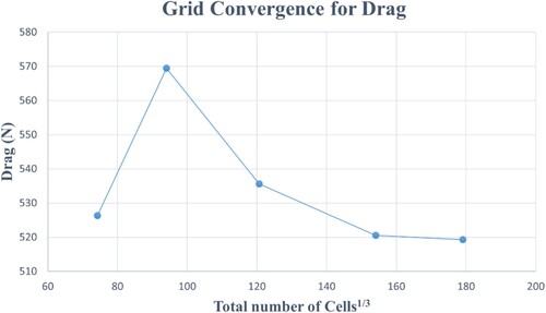
Figure 18. Dependency of heave (rise) and pitch (trim) on mesh size.

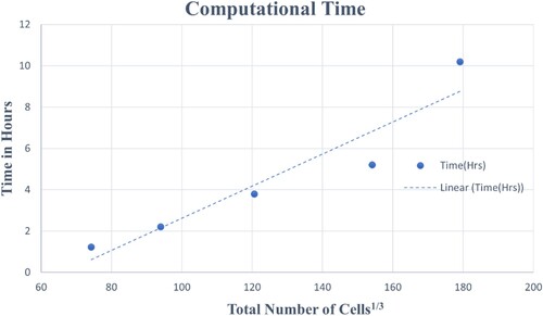
For a good compromise between the solution accuracy and computational effort, computational time is plotted vs. grid size in Figure 19. Computational time is given for an HPC Cluster with 40 cores and 90 GBs of RAM. Time requirements from Mesh 4 to Mesh 5 almost double, with only small improvements in accuracy. Therefore, Mesh 4 with a grid size of 3.6 million cells and computational time of around five hours is thought to be an excellent compromise, particularly for final comparison of results. For an uncertainty analysis see Appendix III.

Figure 19. Simulation time vs. mesh size.

3.6. Validation by comparison to model tests

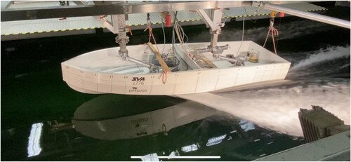
Validation of the chosen CFD set-up is done, additionally, by means of systematic comparisons to a number of experiments undertaken in the towing tank of the Technical University Berlin, see Figure 20 for an impression. For the experimental studies a scale model of length L_PP = 3.364 m was provided by SVA Potsdam. The model features exchangeable tunnel modules and two alternative tunnels are studied.

Figure 20. Model test in TU Berlin’s large towing tank.

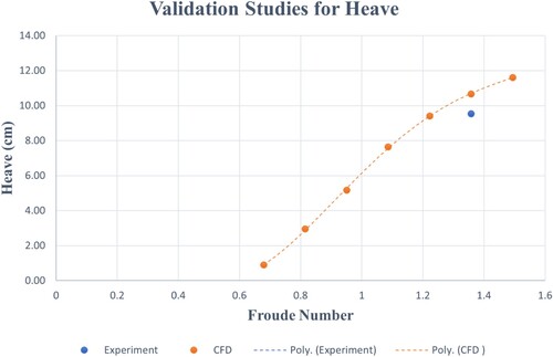
Focus is put on resistance tests to compare numerical and experimental results for drag and running attitude, using Mesh 4. The study is then extended to validate one particular case of self-propulsion by introducing propeller forces in the simulations before starting the optimizations. Table 7 gives the absolute data for various speeds. The results show a very good comparison between numerical simulation and experiments, in particular when considering typical uncertainties for towing tank tests. At design speed of 27.5kn the difference in drag amounts to 0.268% while differences in heave and pitch are 1.14 cm and 0.88 deg at model-scale, respectively. The quality of the simulations is thus assumed to be acceptable.

Table 7. Validation at model-scale for various speeds.

Figures 21–23 show the results from Table 7 for a visual comparison. Resistance is very well captured by the CFD simulation with differences below 1%. For heave and pitch it is more meaningful to compare absolute differences rather than relative values. For pitch the maximum deviation is 0.9 degrees. For heave only one data point is available from the experiments. Here, the difference at model-scale is 1.14 cm at design speed. Taking into account the grid uncertainties discussed above and assuming measurement uncertainties, too, the CFD set-up is considered suitable for optimization.

Figure 21. Comparison of numerical (orange) and experimental (blue) values for resistance (drag).

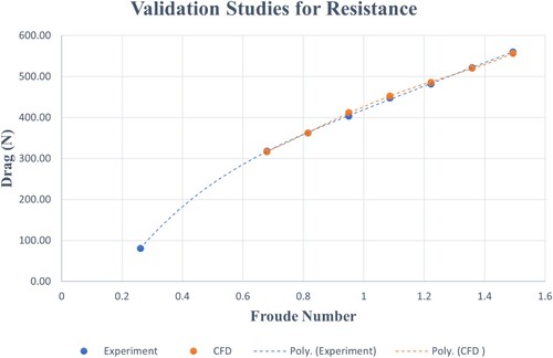
Figure 22. Comparison of numerical (orange) and experimental (blue) values for trim (pitch).

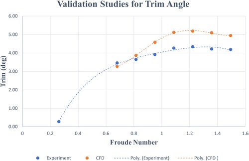
Figure 23. Comparison of numerical (orange) and experimental (blue) values for heave (rise) (only one measurement point available).

4. Simulation-driven design

As introduced in section 1 simulations are used to drive the design process. In order to keep the number of free variables low, the geometry is defined parametrically as presented in section 2. The simulations are undertaken as viscous free surface RANS computations with carefully chosen settings for a good compromise between accuracy and computational resources as discussed in section 3. Propeller thrust is used as the objective to compare designs. The aim is to identify one or several variants whose parameter combinations and resulting shapes provide the lowest thrust, translating to minimum power, at the design speed of V_S = 27.5kn while observing constraints such 9.5ton of displacement, reasonably low trim and good shipbuilding practice. The equality constraint of displacement is readily built into the process, i.e. the boat floats at the draft that yields the correct displacement at rest. The inequality constraint of trim is checked only after the optimizations.

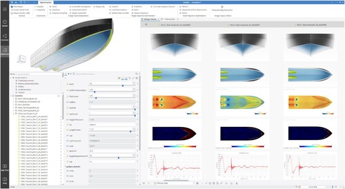
Explorations and exploitations, see Harries (2020), are run directly from CAESES®, using a Java script-based coupling to Simcenter STAR-CCM + via CAESES’ so-called SoftwareConnector. This enables the creation of hundreds of designs without the need of human intervention. Figure 24 illustrates the tight connection. The parametric model can be seen in the top-left window. The mid-left window shows the sliders with which to adjust parameters manually or automatically. Variants produced during one of the optimization campaigns are depicted in the lower-left window, allowing direct access to each of the designs. In the central-right window three geometric variations out of dozens are displayed in CAESES’ so-called DesignViewer. Also shown are pressure plots and volume fraction along with convergence plots as produced by STAR-CCM + and fed back to CAESES.

Figure 24. Variations of geometry and collection of simulation results as summarized in CAESES.

The upcoming sections presents the initial studies, including a search for an optimum position of the longitudinal centre of gravity (LCG), the optimization campaigns and an investigation with regard to the effect of appendages and mesh size on a set of selected designs that are considered close to optimal.

4.1. Manual improvements

Engineering judgement plays an essential role in finding an optimal design, along with utilizing sophisticated optimization engines. Based on a preliminary design by the shipyard a number of manual changes are introduced, such as widening the transom and changing its deadrise, to improve the planing conditions while observing the builder’s design philosophy as well as the expectations of future operators. This established a first baseline selected for model testing and validation.

From both experiments and CFD simulations a certain cross-flow aft of the transom along with higher wave elevations became apparent for the first baseline, complemented by a lower than expected rudder efficiency detected during the tank tests. To resolve these issues and before undergoing extended formal optimizations, the boat’s initial tunnel is modified parametrically and tuned to feature a smoother flow. This is done manually to gain a representative starting point for the actual simulation-driven design process.⁵

The tunnel section being exchangeable in the scale model, a new tunnel is inserted and tank tests are repeated, yielding a smaller wave elevation and a smoother flow. Figure 25 presents the initial and the new tunnel, realized with the parametric model introduced in section 2.3. An impression of the free surface elevations for both tunnels are given in Figures 26 and 27.

Figure 25. Initial tunnel (left) and new tunnel (right), before rotation to position above the propeller (compare to Figure 9).

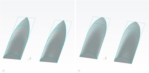
Figure 26. Free surface for planing hull with initial tunnel (first baseline).

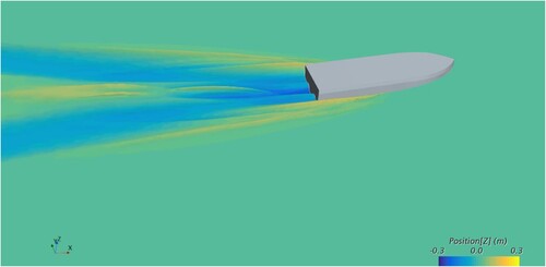
Figure 27. Free surface for planing hull with new tunnel (without pretrim).

Ideally, the new tunnel geometry would already decrease the overall drag force of the vessel. However, the tank tests show rather similar resistance values for both configurations. Utilizing the CFD results, the resistance is decomposed for tangential (shear) and normal components (pressure). A summary is given in Table 8. It can be seen that the pressure drag is decreased for the boat with the new tunnel while the shear drag, coincidently, increases by about the same amount. Thus, the total resistance remains practically the same for both geometries as found in both the experiment and the CFD simulation.

Table 8. Comparison of model-scale data for the boat with the initial and the new tunnel using CFD.

						Drag
	LCG	XCB	Resistance	Trim	Heave	Pressure	Shear
	m	m	N	deg	Cm	N	N
Initial	1.504	1.4681	521.52	5.09	10.06	311.68	209.84
New	1.504	1.4681	520.62	2.98	6.96	263.38	257.24

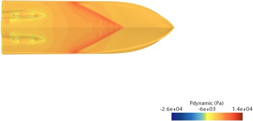
What can also be noted is that the trim angle is much lower for the boat with the new tunnel when compared to the running attitude of the boat with the initial tunnel. In addition, the boat with the new tunnel experiences considerably less rise. Correspondingly, this results in an increase of the wetted surface area of the new geometry. Apparently, the dynamic lift force is lower and the boat stays in a mode closer to semi-planing. Figures 28 and 29 compare the pressure distribution on the hulls for both tunnel configurations.

Figure 28. Pressure distribution for boat with initial tunnel as computed with Simcenter STAR-CCM +.

4.2. Sensitivity analysis for LCG

Fast monohulls are often rather sensitive to the longitudinal position of the centre of gravity (LCG). Their dynamics, trim and heave are directly influenced by the LCG since it directly affects the angle of attack in planing mode. While boats and ships are often designed to float on an even keel when at rest, there might well be an advantage to accept a slight pre-trim to the stern, i.e. bow up.

The pressure distribution in Figure 29 suggests that a backward shift of LCG could increase the running attitude at design speed, gaining better planing characteristics. Table 9 presents the result of a sensitivity analysis for LCG, using the boat with the new tunnel as the basis. At model-scale the LCG position of the vessel is shifted from 1.504 m (default) aftward. It is interesting to take a closer look at the static trim angle. It is small but negative at the initial LCG position. At LCG = 1.468 m, measured from the aft perpendicular (here the transom stern), the longitudinal centre of gravity (LCG) and the longitudinal centre of buoyancy (LCB) are in the same plane and the boat floats without any static trim angle at rest.

Figure 29. Pressure distribution for boat with new tunnel as computed with Simcenter STAR-CCM +.

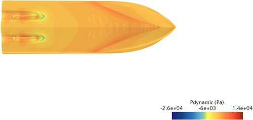
Table 9 . Sensitivity analysis of LCG for boat with new tunnel, using CFD (negative static trim refers to bow down, positive trim means bow up).

LCG	Delta LCG to XCB	Resistance	Running trim	Heave	Pressure drag	Shear drag	Static trim
m	m	N	deg	cm	N	N	Deg
1.504	−0.036	520.62	2.98	6.96	263.38	257.24	−0.22
1.468	0.000	515.01	3.20	7.57	263.29	251.72	0.00
1.454	0.014	511.72	3.26	7.74	261.42	250.30	0.06
1.404	0.064	501.50	3.43	8.34	257.66	243.84	0.23
1.354	0.114	491.80	3.63	8.96	255.30	236.50	0.43
1.254	0.214	478.62	4.02	10.28	258.18	220.44	0.82
1.154	0.314	472.50	4.42	11.74	267.02	205.48	1.22
1.054	0.414	465.18	4.82	13.34	277.92	187.26	1.62

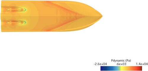
The results of total resistance vs. LCG are plotted in Figure 30, showing a strong correlation. Apparently, shifting the LCG position further aft increases the planing characteristics, decreasing the wetted surface area and the total resistance. Figure 31 depicts the pressure distribution. A wedge-shaped region of high pressure can be seen where the free surface hits the planing surface aft of the bow while the transition between the bare hull and the tunnel features low pressure.

Figure 30. Change of resistance by moving the longitudinal centre of gravity.

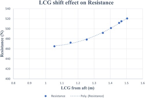
Figure 31. Pressure distribution for boat with new tunnel and LCG shifted aftwards as computed with Simcenter STAR-CCM +.

It is also interesting to plot individual components of the drag force against LCG, see Figure 32. As explained previously, the backward shift of LCG increases the trim angle and decreases the wetted surface area of the vessel, reducing the shear drag. However, the pressure drag only decreases up to a certain point and then begins to go up again.

Figure 32. LCG effect on resistance (drag) components.

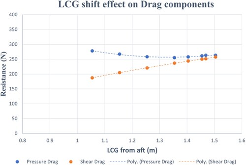
The trends taken from Figures 30 and 32 suggest a parabolic dependency of resistance as a function of LCG. Theoretically, if the LCG was moved further aftward there should be a minimum where the combined effect of both the shear and pressure components yield the lowest total resistance. In practice, the boat’s LCG is limited by design constraints and cannot be moved further towards the stern. Here, at model-scale an LCG shift aft of XCB by 0.114 m, corresponding to a shift of 0.15 m from the initial LCG, is selected as a compromise. At model-scale this gives a LCG of 1.354 m from the AP which translates to 4.45 m at full-scale.

It should be noted that this shift of LCG for the boat with the new tunnel provides an improvement of around 4% in total resistance when compared to the boat with the initial tunnel. This results from standard design processes (SBD) before even starting the SDD campaigns. This configuration – new tunnel and aftward shift of LCG – is taken as the actual baseline for comparisons and is termed ‘new baseline.’ It should be further noted that the boat with the initial tunnel already displays a better performance than the preliminary design. Consequently, the new baseline can be considered a mature hull so that any further improvements should not be attributed to a poor starting point. Note that this ‘new baseline’ also represents the hull selected for full-scale trials.

4.3. Effect of appendages and mesh size

Generating and evaluating hundreds of designs takes many computational hours and resources. In principle, the optimization strategies are employed to produce designs with minimum (or maximum) values of the objectives. Each variant is compared against a reference design, here the new baseline. Improvements are best to be judged by means of relative changes. Potentially, this allows further simplifications to the set-up as long as no detrimental effects on the ranking are introduced.

To check the effect of appendages on the ranking, several designs are generated with a Sobol, a quasi-random DoE sequence, see Harries (2020) for details. Four representative variants are compared to the new baseline by including and omitting appendages. Table 10 summarizes the ranking of designs via an ascending value of drag without considering any appendages. It can be observed that the effect of appendages is to add about 40N to 60N of resistance for each variant. Meanwhile, the heave values increase by around 1 cm and pitch decreases by an average of 0.15 degrees when appendages are present. The actual ranking, however, remains practically the same with and without appendages. The exception is Des0003 when compared to the new baseline. They lie very close together but would just about swap positions. Consequently, it is considered acceptable to undertake the SDD campaigns without appendages which reduces the time for CFD simulations by another 1.5 h per variant. As discussed above simulation time with appendages is about five hours (Mesh 4).

Table 10. Effect of appendages on performance.

	With appendages			Without appendages			Absolute difference
	Resistance	Heave	Pitch	Resistance	Heave	Pitch	Resistance	Heave	Pitch
Design	N	cm	deg	N	cm	deg	N	cm	deg
DesA003	534.27	7.0842	−2.99	476.08	5.8328	−2.77	58.19	1.25	−0.22
New baseline	532.33	6.9755	−2.89	477.64	5.8468	−2.80	54.68	1.13	−0.10
DesA002	537.72	6.9682	−2.90	484.81	5.8924	−2.79	52.90	1.08	−0.11
DesA000	551.98	6.2163	−2.36	500.85	5.2414	−2.23	51.13	0.97	−0.13
DesA001	576.55	5.6768	−1.90	538.55	4.6621	−1.71	38.00	1.01	−0.19

Similar studies are carried out to see the effect of mesh sizes on the design ranking. Table 11 concludes the results of this study for a handful of selected variants. Similar to the study about the omission of appendages, the ranking remains the same for Mesh 4 and Mesh 2, Mesh 4 serving as the ‘yardstick’ from grid convergence as presented in section 3.5. The utilization of Mesh 2 decreases the computational time to 2.5 h from the five hours for Mesh 4. The differences of drag and running attitude show similar trends. Hence, Mesh 2 without appendages is taken for the bulk of the SDD campaigns, reserving the finer mesh and the inclusion of appendages for subsequent quality assessment.

Table 11. Effect of mesh size on performance.

Designs	Mesh 2			Mesh 4			Absolute difference
	Resistance	Heave	Pitch	Resistance	Heave	Pitch	Resistance	Heave	Pitch
	N	cm	deg	N	cm	deg	N	cm	Deg
DesM001	444.49	6.8078	3.31	434.25	6.8590	3.34	10.24	−0.05	−0.03
DesM003	446.40	6.6714	3.32	438.12	6.7170	3.35	8.28	−0.05	−0.03
DesM000	451.22	5.7720	3.22	445.34	5.8646	3.30	5.88	−0.09	−0.07
DesM002	468.86	4.5263	3.10	462.01	4.6536	3.17	6.85	−0.13	−0.07
DesM004	477.78	2.8527	2.94	468.38	3.1885	3.08	9.40	−0.34	−0.15

4.4. SDD campaigns

4.4.1. Overview

Several SDD campaigns are employed, ranging from pure exploration via exploitation to machine learning (ML) and optimization on surrogates. For global exploration the quasi-random sequence by Sobol (1976) is applied while local searches are conducted with the T-search by Hilleary (1966), see also Harries (2020) as well as Birk and Harries (2003).

Figure 33 gives an overview of the SDD campaigns and the designs chosen for a thorough comparison, summarizing the material presented so far: Starting from the preliminary design provided by the shipyard, a manually improved boat with an initial tunnel is created, called first baseline (see section 4.1). Adjusting the tunnel geometry, again manually, a boat follows whose new tunnel yields a better flow in the aftbody but about the same resistance as before. A systematic study of moving the LCG aftward leads to a configuration that is very competitive (see section 4.2) and which is called new baseline. This is considered the first (manually) optimized design and forms the starting point of all successive optimizations.⁶

Figure 33. Overview of the overall design process and the various SDD campaigns (below the dashed line) along with resulting designs.

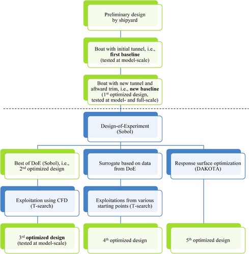
Having coupled Simcenter STAR-CCM + to CAESES® the SDD process commences with a Design-of-Experiment. The best variant form the DoE is named second optimized design from which an additional local optimization is undertaken. For this a deterministic T-search is run which yields the third optimized design. This is the design that is actually model-tested as the ‘optimized design’ upon adjusting the tunnel slightly to fully accommodate the shaft line.⁷

The data from the DoE is utilized to build a surrogate on which several local searches are undertaken, bringing about a fourth optimized design. Moreover, a response surface optimization is conducted, using DAKOTA by Sandia National Laboratories (2023), see also Adams et al. (2021), as integrated in CAESES. This gives a fifth optimized design. The following subsections present further details of the various runs while Table 12 gives an overview of design variables along with their bounds. Variables in the blue box relate to parameters that control the tunnel (a total of 10) while variables in the green box determine the bare hull (a total of eight).

Table 12. Lower and upper bounds of design variables for the SDD campaigns.

4.4.2. Exploration

A Design-of-Experiment is undertaken to explore the 18-dimensional design space globally. The 18 free variables are taken from parameters defining both the bare hull and the tunnel, Table 12. A quasi-random Sobol sequence is utilized for this.

Figure 34 presents the results. The first column shows output parameters of interest, such as thrust, drag, pitch and heave, over the design identifiers. (The numbers are assigned in the sequence of generation within the DoE.) The first row gives thrust in Newtons which represents the objective. Further rows present pitch, heave, RPMs, computational time and other output values of interest. Starting from the second column, each output parameter is plotted against one single design variable. As is apparent from the plots, within a Sobol sequence all design variables change from variant to variant which is different to the systematic change of one parameter at a time typical of an exhaustive search. This is done to explore the design space meaningfully with as few variants as possible, providing the data to identify strong and weak correlations between the objective and the design variables by means of regression analyses and to be able to build surrogates.

Figure 34. Thrust, drag, pitch, heave etc. as functions of several free variables from DoE.

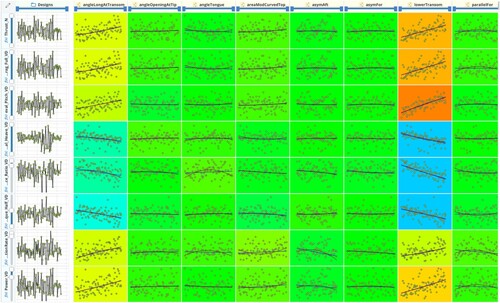
The results of the regression analysis is illustrated via colours in Figure 34 where red indicates a strong positive correlation between the two quantities plotted, i.e. higher values of one quantity are associated, at least in general, with higher values of the other quantity. Blue relates to a strong negative correlation while green shows little to no correlation. Additional correlations between output parameters and the free variables are shown in Figure AIV.1 in Appendix IV.

To better visualize the change of the objective Figure 35 depicts the propeller thrust over the variants generated during the DoE. It is beneficial to plot the difference of the thrust value against the value of the new baseline, a value of 100% representing the starting point of the optimization. Designs having a value of less than 100% are improved variants while designs with values greater than 100% are less competitive. From the changes the design team gets an idea about the room for improvement. Here, quite a few designs already outperform the new baseline, indicating optimization potential.

Figure 35. Change of objective vs. variants in DoE.

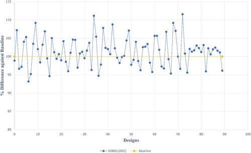
A general recommendation is to test the square of the number of free variables within a DoE in order to develop an appreciation of the design space, see Harries (2020). For higher dimensional spaces also five to 10 times the number of free variables have been reported. Here, a total of 95 variants are investigated since, even though the computational resources needed are heavily reduced already, see sections above, the computational effort per variant is still substantial. Note that for five designs no CFD results could be obtained so that the history shown in Figure 35 runs from 0 to 89, only.

4.4.3. Exploitation

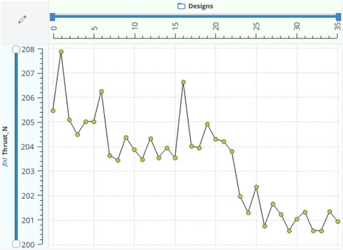
Exploring the design space gives an idea about the location of possible minima. Typically, one or several promising designs from a DoE are taken as starting points for exploitation. Here, design number 15, featuring a thrust that is already about 5% lower than that of the new baseline, is selected from which to commence a T-search in order to find further local improvements.

Limiting the number of additional CFD runs to 35, tangible thrust deductions are brought about by the T-search as depicted in Figure 36. While the first variations within the T-search are small local moves to probe for favourable directions the T-search then walks through the 18-dimensional space with larger steps, ultimately producing an improved variant which is dubbed ‘third optimized design.’⁸

Figure 36. Deterministic optimization via a T-search, starting from DoE’s design number 15 with thrust of one propeller as the objective.

4.4.4. Surrogate

The data generated during the DoE is utilized to train and employ a surrogate, i.e. a response surface model (RSM), for faster predictions without the need to readily perform additional CFD simulations. This can significantly reduce the turn-around times of subsequent optimizations. Typically, either a surrogate is built upfront, provided that the quantity of the simulations available already and the accuracy of the prognosis are sufficient for the design task at hand, or a surrogate is gradually improved with complementing simulations as the surrogate is actually utilized (adaptive sampling).

As thoroughly explained in Ahmed (2022) the data from the Sobol sequence are filtered and various types of trainings are undertaken, yielding good values for the coefficient of determination, i.e. R2-values of around 0.9446.

Figure 37 depicts the optimization history of a local exploitation, again using a T-search, on the basis of the RSM. As can be seen the T-search is run from design number 15 as before. Since the surrogate returns the values of the objective within split-seconds, the T-search is allowed to continue for many iterations. The history depicts the T-search’s characteristic behaviour of small local moves followed by larger steps.

Figure 37. History of the T-search run on the surrogate (grey line) vs. history of the T-search run on the basis of CFD simulations (orange line).

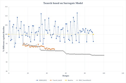
It is interesting to see that there are small discrepancies between the search based on the surrogate and the search based on the CFD simulations. This is due to small differences in the predicted value of the objective. Nevertheless, the intermediate variants from the RSM-based optimization turn out to be quite close to the third optimized design generated purely from CFD, suggesting that they lie on the same ‘plateau’ with differences of one to two percent which can be attributed to the accuracy of the surrogate. Many more variants can be run on the surrogate within just a few seconds, thus allowing a continuation of the search, ultimately leading to further improvements, albeit not yet confirmed by CFD, and a variant called fourth optimized design.

In addition, the surrogate is employed to commence a few more exploitation runs from different starting points, the evaluations not taking a lot of resources. An elaboration is given in Appendix IV.

Utilizing a handful of variants from the optimization on the surrogate, its quality can be checked by evaluating the new shapes with the same CFD set-up originally fed to the machine learning algorithm (ML). Table 13 presents the results of this validation. All the designs are captured well by the surrogate, the maximum deviation between prognosis and simulation being around 2%. This is in line with a general tendency of ML models to slightly overpredict improvements. Very nicely, the order of the variants is kept. The best design found in the optimization on the surrogate remains the best design when employing CFD simulations. Furthermore, designs that lie close to each other in the surrogate remain close in CFD.

Table 13. Validation of the Kriging based ML model.

	Improvements compared to new baseline
Designs from various optimizations	Prediction from surrogate (Kriging)	Order	Simulation with CFD	Order
Starting from new baseline	91.21%	5	93.13%	5
Starting from Des0006	86.21%	1	88.91%	1
Starting from Des0015 (3^rd optimized design)	88.11%	3	90.05%	3
Starting from Des0038	86.36%	2	89.36%	2
Starting from Des0070	89.13%	4	90.39%	4

4.5. Selected results

4.5.1. Hydrodynamics

From the various SDD campaigns, exploring and exploiting the 18-dimensional design space globally and locally, several promising designs are identified. See again Figure 33 for an overview.

It is of interest to compare the improvements achieved along with the resources spent as compiled in Table 14. To recap, the 1^st optimized design corresponds to the new baseline derived manually from a first baseline. The 2^nd optimized design is design number 15 taken from the Design-of-Experiment. Starting from there, a T-search produced the 3^rd optimized design, always using CFD simulations for each new step. This, naturally, took a lot of additional resources and constitutes the most ‘expensive’ approach. The 4^th optimized design employs a surrogate based on the data from the DoE and stems from running local exploitations. Finally, the 5^th optimized design is found from one of DAKOTA’s algorithms.

Table 14. Summary of optimization results.

Optimized design	Optimization method	Propeller thrust	Difference to new baseline	CPU time spent	Data set utilized
		N	%	Hours	hours
1^st	New baseline	436.84	100.00	2.3	–
2^nd	Best of DoE (Sobol)	413.42	94.64	207	–
3^rd	Best from exploitation using CFD (T-search)	401.88	92.00	80.5	207
4^th	Best from surrogate (T-search-RSM)	393.36	90.05	2.3	207
5^th	Best from DAKOTA based on DoE	391.12	89.53	2.3	207

The DoE takes up most of the computational time as can be expected. The additional time associated with the 1^st, the 4^th and the 5^th optimized design, respectively, corresponds to a single additional CFD simulation, in case of the 4^th optimized design for validation and in case of the 5^th optimized design for validation and improvement of the surrogate. It should be kept in mind, of course, that the 1^st optimized design stems from an educated yet somewhat lucky guess.

The optimization results presented in Table 14 are based on the fastest possible CFD set-up as discussed above. In order to double-check the quality achieved all optimized designs are rerun with a finer mesh and as appended models (albeit, again without rudders). The results are given in Table 15. It can be seen that, combining different optimization approaches, improvements between a bit more than 8% compared to the first baseline up to almost 20% could be realized with regard to thrust as the objective. Naturally, it should be kept in mind that large improvements should cautiously be attributed to a reasonably good yet not mature baseline.

Table 15. Optimization Results for Appended Model with Finer Mesh.

		Optimized designs
	First baseline (tested at model-scale)	1st, i.e. new baseline (tested at model- and at full-scale)	2nd	3rd (tested at model-scale)	4th	5th	Units
Thrust	542.26	494.78	448.6	440.76	434.64	438.34	N
Rotational speed of prop.	2320.5	2255.47	2204.2	2205.83	2205.12	2199.32	rpm
Torque	25.18	23.46	21.42	21.196	20.9644	21.0506	Nm
Power	3.0587	2.7705	2.4721	2.4481	2.4205	2.4241	kW/engine
Pitch	5.85	4.21	3.83	4.57	4.556	5.01	deg
Heave	0.1231	0.0975	0.09	0.1038	0.1047	0.1134	m
LCG	1.504	1.354	1.354	1.354	1.354	1.354	m
Improvement	0.00%	8.76%	17.27%	18.72%	19.85%	19.16%

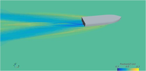
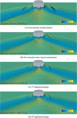
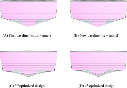
The wave fields of the new baseline and of two of the optimized designs – i.e. the 3^rd optimized design and the 4^th optimized design – are shown in Figures 38–40. They can be directly compared to the wave fields given in Figures 26 and 27. Furthermore, Figure 41 presents the wave field for selected designs from a stern view, again as computed with Simcenter STAR-CCM +. The reduction in wave height from the first baseline via the new baseline to the 3^rd and the 4^th optimized designs is apparent. Differences in the wave pattern are particularly pronounced directly aft of the transom.

Figure 38. Free surface for new baseline (new tunnel with pretrim) (also compare to Figures 26 and 27).

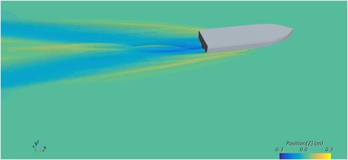
Figure 39. Free surface for 3^rd optimized design (also compare to Figures 26 and 27).

Figure 40. Free surface for 4^th optimized design (also compare to Figures 26 and 27).

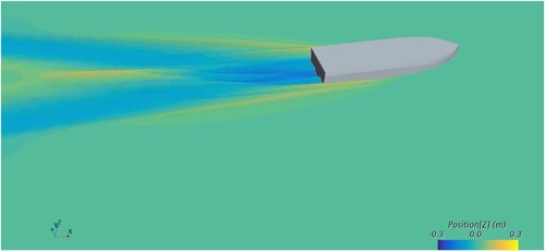
Figure 41. Stern views of wave fields for selected designs.

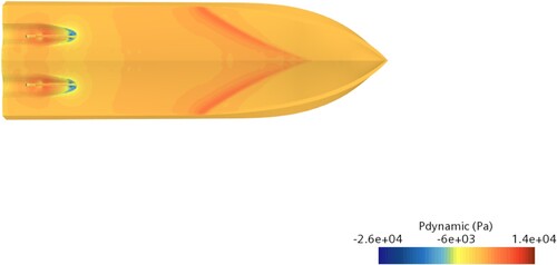
In addition and to allow a comparison to Figures 28–30, Figure 42 depicts the pressure distribution of the 3^rd optimized design. All pressure plots nicely show the high pressure region in the forebody along with low pressure regions at the transition from the hull to the tunnel. It can be readily appreciated that the location and shape of the high pressure regions differ between the various designs.

Figure 42. Pressure distribution for 3^rd optimized design as computed with Simcenter STAR-CCM + (also compare to Figures 28 and 29).

4.5.2. Geometry

A comparison of the geometry is presented for four selected designs that are identified throughout the SDD campaigns as being of particular importance: The first baseline, the new baseline (1^st optimized design), the 3^rd optimized design and the 4^th optimized design, see also Table 15. Based on a joint analysis by all parties involved the 3^rd optimized design is chosen for additional model-tests as it yields excellent improvement and also reflects the shipyard’s design preference. The 4^th optimized design is presented, too, as it yields the highest improvements. Figures 43–46 showcase the geometries in perspective, side, bottom and transom view, respectively. An additional bow view is given in Appendix IV along with a spider plot of free variables that yield low propeller thrust.

Figure 43. Perspective view of selected designs.

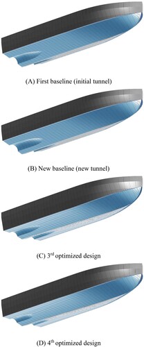
Figure 44. Side view of selected designs.

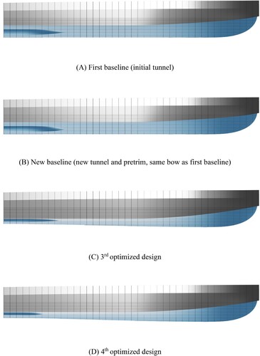
Figure 45. Bottom view of selected designs.

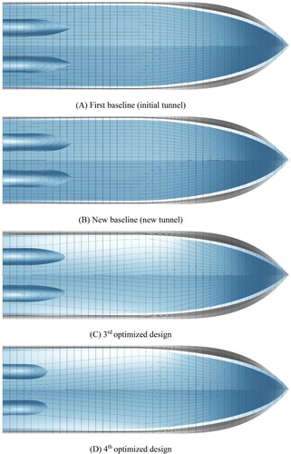
Figure 46. Transom view of selected designs.

It can be noted that the initial and the new baseline differ in the tunnel only. Also, the waterlines and sections of both baselines are rather straight in the planing region aft of midship. This is altered for the two optimized variants. The optimization leads towards a reduction in deadrise, introduces a tangible rocker and yields a certain hollowness in the sections.

The tunnel of both the 3^rd optimized design and the 4^th optimized design is less pronounced as a consequence while the transom lies slightly deeper in the water at rest. The length of the tunnel of the 4^th optimized design is quite a bit shorter. This implies that the shafts protrude in front of the tunnel and not, as with both baselines and the 3^rd optimized design (albeit in a subtly modified version), within the tunnel itself, excluding it from final selection.

5. Off-design conditions and outlook

5.1. Performance at different operating conditions

As stated in section 3.1, during the optimizations propeller thrust at design speed and at design displacement is used as a single objective. Naturally, the pilot boat will not only run at this ideal condition but within a range of speeds and at various displacements. Therefore, the performance of the performance is also studied at these off-design conditions.

Figure 48 depicts the propeller thrust, computed via STAR-CCM + at model-scale, as a function of speed for three displacements, namely design displacement of 9.5ton and two higher displacements of 10ton and 10.5ton, respectively. A comparison is given between the performance of the new baseline (crosses as markers) and the 3^rd optimized design (dots as markers).

It can be nicely seen from Figure 47 that the 3^rd optimized design outperforms the new baseline at all displacements and at all speeds. The optimized design at 10.5ton even outperforms the new baseline at 9.5ton. Interestingly, the slopes of the thrust-speed curves are slightly lower for the optimized design than for the new baseline, in particular at the design speed of 27.5kn. It can thus be concluded that, even though the 3^rd optimized design stems from a single-objective optimization, it constitutes a rather robust optimum (for the chosen objective of thrust) that does not show any rapid deterioration at off-design conditions.

Figure 47. Propeller thrust at model-scale vs. speed for the new baseline and the 3^rd optimized design at three representative displacements.

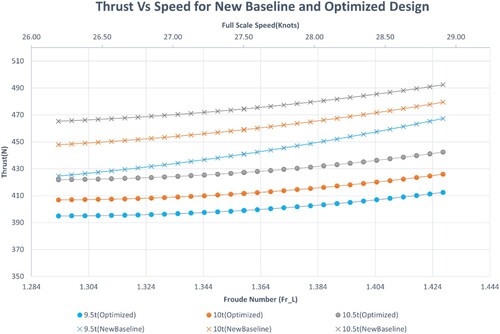
It should be noted that for the analyses presented in Figure 47 a surrogate is utilized for each of the designs. The surrogates are based on CFD simulations for quasi-randomly chosen combinations of displacement, trim and speed, produced by a Sobol sequence as a DoE. The thrust-speed curves are then derived by evaluating the surrogates. This approach reduces the number of simulations required to determine the thrust necessary at any planing condition of interest without the need of additional CFD runs.

5.2. Outlook

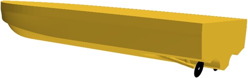
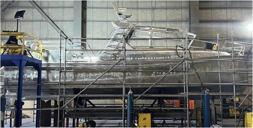
Within the R&D project AutoPlan many tasks are undertaken that could not all be covered within this paper. In the context of the material presented here, they concern further model test campaigns and full-scale sea trials to improve the understanding of the hydrodynamics of planing boats, not only in calm water at a straight course but also with respect to maneuvering. To this end, a full-scale prototype is realized by UZMAR, see Figure 48. It is built in aluminium and features the lines of the new baseline.

Figure 48. Full-scale prototype being built at UZMAR (photo courtesy of Nalan Erol, AutoPlan project coordinator).

Furthermore, several optimization campaigns are conducted like SDD on the basis of dimensionality reduction, see Ahmed (2022), and by employing alternative optimization algorithms. Also, comprehensive model-scale tests are undertaken with the 3^rd optimized design at the Technical University Berlin, to be reported at a later point of time along with a systematic comparison between simulations and experiments. Preliminary evaluations of the measurements already confirm that the 3^rd optimized design indeed performs better than the new baseline.

Moreover, the many CFD simulations performed during the exploration and exploitation phases can be utilized to develop a reduced-order model (ROM) that not only allows predicting the performance of a new variant with respect to thrust but that nicely provides pressure plots on the wetted surface of the hull and wave patterns, see Ahmed et al. (2023). This holds the potential of supplying a design team with direct access to information about both energy consumption and flow fields.

Naturally, there are further options to decrease the energy consumption of the boat beyond the gains achieved so far. For instance, inner spray rails can be utilized, see Larsson et al. (2014). Trim flaps or interceptors could be introduced, too, so as to optimize the running trim at different speeds. It should be noted, however, that the intention of this paper is not to propose the best planing boat possible but rather to elaborate on all elements of a thorough SDD project.

6. Conclusions

The paper presents the simulation-driven design of a fast monohull. The boat is 11 m in length and developed for a design speed of 27.5kn at a displacement of 9.5ton, making it a hull at the lower end of planing (Section 1). The hydrodynamic design is realized within the R&D project AutoPlan by a team of experts from a shipyard (UZMAR), a software developer specializing in SDD (FRIENDSHIP SYSTEMS), hydrodynamicists from a university (TU Berlin) and a model basin (SVA Potsdam).

A versatile fully parametric model for the bare hull and the tunnel, using CAESES, is described (Section 2). It combines parametric models for the bare hull and the tunnel which are assembled by means of a Boolean operation. 18 parameters of the model are chosen as free variables for various SDD campaigns. The free variables can be independently changed, always yielding a fair and watertight geometry, ready for CFD analysis.

A suitable set-up for RANS simulations including heave and trim as well as the influence of the propellers, using Simcenter STAR-CCM+, is discussed (Section 3). A thorough comparison between simulations and experiments confirms the applicability of the numerical model. The turn-around time for the RANS simulations is systematically reduced in order to come up with reasonably fast yet meaningful results for the ranking of variants (Section 4). This is an important prerequisite for SDD: The relative changes of performance need to be captured while many variants need to be investigated within the available period of time. It is shown that a coarser mesh and omitting the appendages are acceptable to run the bulk of the simulations. Subsequently using a finer mesh and taking the appendages into account confirms that the various designs identified as optimal are indeed better than the baseline (Section 4).

Based on the shipyard’s preliminary design, targeting the service profile as a pilot boat and considering constraints of production and operation, several changes are introduced manually, yielding a first baseline and, based on a systematic study on pre-trim, a new baseline (Section 4). This new baseline stems from simulation-based design (SBD) and can be considered competitive. Due to the timeline of the R&D project the shipyard chose to build this hull at full-scale.

Several optimization campaigns are run from the new baseline. They include explorations and exploitations to understand the design space and to improve the planing boat with regard to thrust as the objective, respectively. A classic Design-of-Experiments (DoE) yields an understanding of the potential for improvements, correlations between the objective and free variables and, importantly, the input data for a surrogate. Even though the design space is 18-dimensional, 90 variants suffice to produce a surrogate that is good enough for further simulation-driven design (SDD). Different optimization strategies are put to use, mainly deterministic searches set off from DoE-variants found to be better than the new baseline already. Several variants are identified that decrease the thrust needed at design speed by almost 20% when compared to the first baseline, representative of good naval architecture practice without the benefit of using CFD. One optimized design is selected for further numerical and experimental investigations. This design outperforms the new baseline over a wide range of operating conditions, proving that a robust solution is proposed (Section 5).

The paper presents a thorough SDD campaign and explains all the necessary steps. It is shown that substantial gains can be realized by running systematic explorations and formal exploitations even if tangible manual improvements have already been made.

Abbreviations

Table

AutoPlan	European R&D project, www.auto-plan.net
BRep	Boundary representation
B-spline	Basis spline
CAD	Computer Aided Design
CAESES^®	Computer Aided Engineering System Empowering Simulation, see www.caeses.com (accessed February 3, 2023)
CFD	Computational Fluid Dynamics
CoG	Centre of gravity
curveEngine	Pattern for the fully parametric definition of curves
DoE	Design-of-Experiment (exploration of a design space)
DoF	Degree-of-Freedom (number of free variables)
Fn	Froude number based on length of the waterline at rest
FnB	Froude number based on beam at transom at rest
Fn∇	Froude number based on displacement
FS	Richardson extrapolation factor of safety
GCI	Grid convergence index
HRIC	High resolution interface capturing scheme
INA	Intelligent Navigation System
IPR	Intellectual Property Rights
ITTC	International Towing Tank Conference
MetaSurface	Fully parametrically defined sweep surface
ML	Machine learning
NURBS	Non-Uniform Rational B-Spline
R	Refinement ratio (grid dependency study)
R&D	Research and development
RANS solver	Reynolds-Averaged Navier-Stokes solver
ROM	Reduced order model
RT	Total resistance, drag
ruledSurface	Surface defined as a linear blend between two curves (rails)
SBD	Simulation-based design
SDD	Simulation-driven design
SIMPLE	Semi-implicit method for pressure-linked equations
STAR-CCM+	RANS code within Siemens Simcenter, see www.plm.automation.siemens.com/global/en/products/simcenter/STAR-CCM.html (accessed February 3, 2023)
STEP	Standard for the Exchange of Product Model Data
T	Thrust
TP	Towing point
VOF	volume-of-fluid
webApp	Web-based application (microservice)
WEGEMT	European Association of Universities in Marine Technology
2d	Two-dimensional (planar)
3d	Three-dimensional
1-DoF	One degree-of-freedom (e.g. surge only)
2-DoF	Two degrees-of-freedom (e.g. sinkage and trim)
3-DoF	Three degrees-of-freedom (e.g. surge, trim and rise)

Acknowledgements

The MarTERA project AutoPlan (www.auto-plan.net) brings together partners from Germany, Turkey and Italy. From Germany these are FRIENDSHIP SYSTEMS (www.friendship-systems.com), Schiffbau-Versuchsanstalt Potsdam (SVA, www.sva-potsdam.de) and Technical University Berlin (TU Berlin, www.tu-berlin.de) while from Turkey these are Piri Reis University (www.pirireis.edu.tr), Offshore Engineering Solutions (OES, www.oesdenizcilik.com) and UZMAR (uzmar.com) plus, as associated partner from Italy, Consiglio Nazionale delle Ricerche – Institute of Marine Engineering (CNR-INM, www.inm.cnr.it). The authors would like to thank their colleagues from these organizations, in particular, Nalan Erol from UZMAR for leading the AutoPlan project and Prof. Dr. Andrés Cura from TU Berlin for conducting the towing tank tests with his team, using a scale model built at SVA Potsdam. From FRIENDSHIP SYSTEMS we would like to thank Claus Abt and Carl Benz for their support in parametric modeling and grid generation, respectively. Finally, from Siemens we would like to thank Dr. Miles Wheeler, Aaron Godfrey and Dr. Dejan Radosavljevic for their support throughout the project, in particular for sharing their know-how of running numerical flow simulations for planing boats.

Disclosure statement

No potential conflict of interest was reported by the author(s).

Additional information

Funding

Parts of the work presented in this paper were realized within the research and development project AutoPlan (Automatic Navigation Assistance System for Planing and Semi-planing Crafts), funded by the Federal Ministry for Economic Affairs and Climate Action (BMWK) on the orders of the German Bundestag and PtJ as the conducting agency [FKZ 03SX523A].

Notes

1 The engines ordered by the shipyard, however, are expected to allow for higher speeds. At 32kn and for a displacement of 9.5ton the volumetric Froude number reaches 3.63 at which point this criterion would be fully met, too

2 Harries et al. (2015) presents on overview of the various approaches of parametric modeling, distinguishing fully-parametric and partially-parametric modeling. The former assumes that the entire shape of interest is determined by parameters. The latter is built on existing shapes, wherever they may come from, and just uses parameters to evoke local modifications, for instance, by means of radial basis functions as presented in Harries and Uharek (2021). Hybrid modeling approaches combine the better of the two worlds, depending on the modeling task at hand.

3 An appreciation of the model can be gained interactively from the corresponding webApp at www.friendship-systems.com/products/web-apps

4 also known as Chimera grid

5 and to make reaching any further improvement challenging

6 Everything shown above the dashed line in Figure 33 can be considered simulation-based design while the various processes and results below the dashed line should be seen as simulation-driven design.

7 The subtle elongation of the tunnel is investigated numerically via a systematic change which shows no detrimental effects of performance.

8 This design is model-tested, too, for comparison to the new baseline.

References

- Adams BM, Bohnhoff WJ, Dalbey KR, Ebeida MS, Eddy JP, Eldred MS, Hooper RW, Hough PD, Hu KT, Jakeman JD, et al. 2021. Dakota, A Multilevel Parallel Object-Oriented Framework for Design Optimization, Parameter Estimation, Uncertainty Quantification, and Sensitivity Analysis. Version 6.15 User’s Manual. Sandia Technical Report SAND2020-12495.
- Ahmed O. 2022. Speeding-Up simulation driven design for high-speed planing boat [master thesis]. École Centrale de Nantes.
- Ahmed O, Harries S, Lohse J, Salecker S-E. 2023. Parametric modeling, CFD simulations, DoE and machine learning for the design of a planing boat. Conference on computer applications and information technology in the maritime industries (COMPIT 2023), Drübeck, Germany.
- Albert S, Harries S, Hildebrandt T, Reyer M. 2016. Hyrodynamic optimization of a power boat in the cloud. High-Performance marine vehicles (HIPER 2016), Cortona, Italy.
- Albert S, Hildebrandt T, Harries S, Bergmann E, Kovacic M. 2021. Parametric modeling and hydrodynamic optimization of an electric catamaran ferry based on radial basis functions for an intuitive Set-up. Conference on computer applications and information technology in the maritime industries (COMPIT 2021), Tullamore, Ireland.
- Birk L, Harries S. 2003. OPTIMISTIC – Optimization in Marine Design. 39th WEGEMT, Mensch & Buch Verlag. ISBN 3-89820-514-2.
- Blount D. 2023. Design of Propeller Tunnels for High-speed Craft. [accessed 2023 January 31]. https://www.boatdesign.net/.
- Harries S. 1998. Parametric design and hydrodynamic optimization of ship hull forms. [PhD thesis]. Technical University Berlin, Mensch & Buch Verlag. ISBN 3-933346-24-X.
- Harries S. 2020. Practical shape optimization using CFD: state-Of-The-Art in industry and selected trends. Conference on computer applications and information technology in the maritime industries (COMPIT 2020), Pontignano, Italy.
- Harries S, Abt C. 2019a. Faster turn-around times for the design and optimization of functional surfaces. Ocean Eng. 193:106470. Elsevier. doi:10.1016/j.oceaneng.2019.106470.
- Harries S, Abt C. 2019b. The holiship platform for process integration and design optimization. In: A. Papanikolaou, editor. A holistic approach to ship design – Vol. 1: optimisation of ship design and operation for life cycle. Springer.
- Harries S, Abt C, Brenner M. 2015. Upfront CAD – parametric modeling techniques for shape optimization. international conference on evolutionary and deterministic methods for design, optimization and control with applications to industrial and societal problems (EUROGEN 2015). In: Published by E. Minisci, editor. Advances in evolutionary and deterministic methods for design, optimization and control in engineering and sciences. Glasgow, UK: Springer; p. 191–211.
- Harries S, Uharek S. 2021. Application of radial basis functions for partially-parametric modeling and principal component analysis for faster hydrodynamic optimization of a catamaran. J Mar Sci Eng. 9(10):1069. doi:10.3390/jmse9101069.
- Hess JL, Smith AMO. 1962. Calculation of the Non-lifting potential flow about arbitrary three-dimensional bodies. Report No. E.S. 40622. Long Beach: Douglas Aircraft.
- Hilleary R. 1966. The tangent search method of constrained minimization. In: tech. Rep./Res.paper 59. Monterey: United States Naval Postgraduate School.
- ITTC. 2014. ITTC – Recommended Procedures and Guidelines, Practical Guidelines for Ship Self-Propulsion CFD, 7.5–03–03–01.
- Larsson L, Eliasson RE, Orych M. 2014. Principles of yacht design. International Marine/McGraw-Hill Education, Camden, Maine, USA. 4th ed. ISBN 978-0-07-182640-2.
- Lin W-C, Webster WC, Wehausen JV. 1963. Ships of minimal total resistance. Proc. Int. seminar on wave resistance, University of Michigan, Ann Arbor, MI, USA.
- Nowacki N. 1963. Potentialtheoretische Strömungs- und Sogberechnungen für schiffsähnliche Körper [PhD Thesis]. Berlin: Technical University.
- Nowacki N. 2003. Design synthesis and optimization – An historical perspective. 39th WEGEMT, Mensch & Buch Verlag, 1–26. ISBN 3-89820-514-2.
- Papanikolaou A. 2024. On parametric modeling, digital siblings and ship design optimisation. Ship Technology Research – Schiffstechnik. To be Published.
- Pien PC, Moore WL. 1963. Theoretical and experimental study on wave-making resistance of ships. In: Proc. Int. seminar on wave resistance. Ann Arbor, MI, USA: University of Michigan.
- Sandia National Laboratories. 2023. DAKOTA – Reference Manual [accessed 2023 February 24]. https://dakota.sandia.gov/content/612-reference-manual.
- Savitsky D. 1964. Hydrodynamic design of planing hulls. Mar Technol. 1/1:71–95.
- Savitsky D, Brown PW. 1976. Procedures for hydrodynamic evaluation of planing hulls in smooth and rough water. Mar Technol. 13/4:381–400.
- Sobol IM. 1976. Uniformly distributed sequences with an additional uniform property. Zh. vych. Mat. Mat. Fiz. 16: 1332–1337 (in Russian). U.S.S.R. Comput. Maths. Math. Phys. 16:236–242. (in English).
- Wheeler MP, Matveev KI, Xing T. 2021. Numerical study of hydrodynamics of heavily loaded hard-chine hulls in calm water. Journal of Marine Science and Engineering. 9:2. doi:10.3390/jmse9020184.
- Xing T, Stern F. 2010. Factors of safety for Richardson extrapolation. J Fluids Eng. 132:061403. doi:10.1115/1.4001771.