Reconstructing higher-resolution four-dimensional time-varying volumetric data

Abstract

We have witnessed substantial growth in super-resolution research within the computer vision community. Unlike previous works that mainly focus on the super-resolution synthesis of images, videos, or single volumes, our research is dedicated to the super-resolution synthesis of time-varying volumetric data, which are generated from scientific simulations and are crucial for domain scientists to understand and analyse complex scientific phenomena. Compared to previous works, our research presents a greater challenge: the time-varying volumetric data have higher dimensions, making it more difficult to synthesise super-resolution that maintains good spatio-temporal consistency while achieving high visual quality. To tackle this challenge, we introduce a new GAN-based network called SSR-DoubleUNetGAN, which includes novel network architecture and loss functions, allowing for accurate synthesis of spatial super-resolution for time-varying volumetric data with relatively fast training time. Our method can be applied in the context of in-situ visualisation to aid domain scientists in analysing more time-varying volumetric data more efficiently. In addition, it can be used in the compression-decompression pipeline to recover the super-resolution time-varying volumetric data from their low-resolution counterpart. To demonstrate its effectiveness, we applied various time-varying volumetric datasets from different scientific simulations to it. To demonstrate its advantages, we compared it qualitatively and quantitatively with five state-of-the-art super-resolution techniques, namely SSR-TVD, Tricubic, SRResNet, Cubic, and Linear. Furthermore, we conducted an ablation study to validate its important modules. The experimental results show that our method outperforms the compared state-of-the-art techniques.

Keywords:

• Generative adversarial network
• deep learning
• super-resolution
• time-varying volumetric data

1. Introduction

Super-resolution refers to a technique that can transform low-resolution data with small dimensions into high-resolution data with larger dimensions, using a given scale factor. For example, given a scale factor of $4\times 5\times 6$ (where 4, 5, and 6 denote the scale factors in the x, y, and z dimensions, respectively), the super-resolution technique could transform low-resolution volumetric data with dimensions of $32\times 32\times 32$ to high-resolution volumetric data with dimensions of $128\times 160\times 192$. It has been a very important research topic over the last two decades and has been applied to a wide range of real-world problems in various application domains, such as satellite and aerial imaging (Yuan et al., 2011; Zhang, Zhang et al., 2012), medical image processing (Greenspan, 2009; Gu et al., 2020; Huang et al., 2017), facial image analysis (Zhang, He et al., 2012; Zou & Yuen, 2011), surveillance and security (Rasti et al., 2016; Zhang et al., 2010), sign and number plate reading (Zhang, Jiang et al., 2012; Zhou et al., 2012), and biometric recognition (Begin & Ferrie, 2007; Reibman et al., 2006), to name a few.

On the other hand, conducting research on the super-resolution synthesis of time-varying volumetric data is of great importance in the scientific visualisation community. This is because the computing power of supercomputers has rapidly advanced. As a result, the time-varying volumetric data generated from scientific simulations on supercomputers tend to have larger scales e.g. petascale or even exascale (Shan et al., 2013), span longer time steps e.g. thousands of time steps, and contain more variables with different types e.g. scalar, vector, and tensor. Accurately analysing and visualising these time-varying volumetric data can effectively help domain scientists understand and gain insight into the various time-dependent phenomena behind the data. However, due to the limitations of I/O speed and storage capacity, scientists can only sparsely store the time-varying volumetric data in practice (e.g. sample a small portion of the data) for post hoc analysis and visualisation. Unfortunately, the limitations seriously hinder their ability to study and understand these phenomena. The research on super-resolution synthesis of time-varying volumetric data can address this issue by incorporating it into in-situ visualisation. For example, during the simulation, scientists could adjust the parameters in order to generate low-resolution time-varying volumetric data with smaller sizes. Then, during the post hoc analysis, they can reconstruct the super-resolution from the low-resolution data. In this way, we enable scientists to analyse more data more quickly.

In recent years, with the rapid development of deep learning techniques, the research on super-resolution has gained significant momentum. We have witnessed remarkable progress in the state-of-the-art methods and their performance on various benchmarks. However, most of these studies focus on the super-resolution synthesis of images, videos, and volumetric data. Few studies have specially addressed the super-resolution synthesis of time-varying volumetric data. In comparison to images, videos, and volumetric data, time-varying volumetric data have higher dimensions and are therefore more complex in terms of time and space. Directly extending those super-resolution methods designed for images, videos, and volumetric data to time-varying volumetric data may result in inaccurate super-resolution results that lack fine details. Figure 11 illustrates this with an example. In this example, the SRResNet is a technique that was originally used for super-resolution synthesis of images and has now been extended for super-resolution synthesis of time-varying volumetric data. In comparison to the ground truth results, we can see that the synthesised super-resolution results from the SRResNet lack details e.g. the pointy top located on the right side of the ground truth becomes less pointy, and some internal features of the ground truth appear blurry or are even missing.

To address the above-mentioned problem, this paper proposes a novel method called SSR-DoubleUNetGAN (Spatial Super-resolution Double UNet Generative Adversarial Network). This method utilises the technique of GAN to accurately synthesise the spatial super-resolution of time-varying volumetric data, while also maintaining a good temporal coherence in consecutive time steps. In short, the research makes the following contributions: firstly, we propose the SSR-DoubleUNetGAN method, which incorporates innovative network architectures and loss functions, and can be utilised to synthesise super-resolution of the time-varying volumetric data that is 64 or 125 times larger. Secondly, we apply several time-varying volumetric datasets from various scientific simulations to demonstrate the effectiveness of our method. We conduct both qualitative and quantitative experiments to showcase the advantages of our method compared to other state-of-the-art techniques. Third, we conduct an ablation study to validate the effectiveness of several crucial modules in SSR-DoubleUNetGAN.

The industrial significance of our research is twofold: firstly, it can be used in the in-situ visualisation setting to assist domain experts in analysing more time-varying volumetric data more efficiently. Specifically, during the simulation, spatial low-resolution time-varying volumetric data are generated. In this way, it can achieve faster output speed while generating more data (this is because, unlike spatial high-resolution time-varying volumetric data, spatial low-resolution data occupy less storage space). During the postprocessing stage, we utilise our method to recover spatial low-resolution time-varying volumetric data into spatial high-resolution data for analysis and visualisation purposes. Secondly, it can fit into the compression-decompression pipeline, where time-varying volumetric data are compressed first and then decompressed.

2. Related works

2.1. Deep learning-based super-resolution synthesis

Deep learning techniques have achieved great success in super-resolution synthesis. We recommend that readers refer to Wang et al. (2021) and Lepcha et al. (2023) for a comprehensive review. We divided the research on super-resolution into subcategories based on the types of data used.

2.1.1. Image super-resolution

Most of the super-resolution works focus on images, including both natural and medical images. Here, we will only review the research on super-resolution that is relevant to natural images. For research on super-resolution relevant to medical images, we review it in Section 2.2. Ledig et al. (2017) proposed a super-resolution generative adversarial network (SRGAN), which is the first framework capable of generating photo-realistic natural images with a scaling factor of $4\times$. The novelty of their work is that they define a novel perceptual loss using high-level feature maps from the VGG network combined with a discriminator that encourages solutions perceptually hard to distinguish from the high-resolution reference images. However, hla limitation of their work is that the SRGAN variants of deeper networks are increasingly difficult to train due to the appearance of high-frequency artefacts. Zhang et al. (2018) proposed a very deep residual channel attention network (RCAN) to achieve better single-image super-resolution results. Their work has two main contributions: firstly, they introduce residual in residual (RIR) structure that allows to construct very deep trainable networks; secondly, they introduce a channel attention (CA) mechanism to adaptively re-scale features by considering interdependencies among feature channels. One shortcoming of the RCAN is its high computational complexity compared to other frameworks, e.g. Lai et al. (2017). Tong et al. (2017) presented a novel single-image super-resolution method by introducing dense skip connections in a very deep network. The key contribution of this work is that the feature maps of each layer are propagated into all subsequent layers, providing an effective way to combine the low-level features and high-level features to boost the reconstruction performance. In addition, the dense skip connections in the network enable short paths to be built directly from the output to each layer, alleviating the vanishing-gradient problem of very deep networks. One minor shortcoming of the proposed network is that it does not take the perceptual loss into account to reconstruct photo-realistic high-resolution images. Li, Yang et al. (2019) proposed an image super-resolution feedback network (SRFBN) to refine low-level representations with high-level information. Specifically, they use hidden states in a recurrent neural network (RNN) with constraints to achieve such feedback manner. A feedback block (FB) is designed to handle the feedback connections and to generate powerful high-level representations. The proposed SRFBN comes with a strong early reconstruction ability and can create the final high-resolution image step by step. Furthermore, they introduce a curriculum learning strategy to make the network well-suitable for more complicated tasks, where the low-resolution images are corrupted by multiple types of degradation. To address the issue that the current deep learning-based super-resolution methods remain unsatisfactory in recovering the high-frequency edge details of the images in noise-contaminated imaging conditions, Jiang, Wang, Yi, Wang, Lu, et al. (2019) proposed a GAN-based edge-enhancement network (EEGAN) for robust satellite image super-resolution reconstruction along with the adversarial learning strategy that is insensitive to noise. The experimental results show that their method can reconstruct sharp edges and clean image contents, more realistic and faithful to the ground truth. In addition, they proposed a hierarchical dense connection recursive network (HDRN) (Jiang et al., 2020) to establish a realistic mapping between the low-resolution and high-resolution images. This model incorporates two key modules: one is the hierarchical dense block (HDB), which is used to promote the feature representation while saving the memory footprint with a hierarchical matrix structure design; The other one is the global fusion module (GFM), which is used to fuse all the complementary feature maps. Moreover, they presented a simple but effective adaptive-threshold-based multi-model fusion network (ATMFN) (Jiang, Wang, Yi, Wang, Gu, et al., 2019) to construct the super-resolution of the tiny and compressed face images. Unlike previous methods that learn prior knowledge for the parameters of one statistical model or the desired high-resolution images, their method employs multiple candidate deep-learning networks (CNN, GAN, and RNN) to exploit the ensemble learning superiority, and thus can generate creditable facial contours as well as clear contents. Recently, diffusion model (DM) has shown state-of-the-art results in image and speech synthesis (Chen, Zhang et al., 2021), and some diffusion frameworks have been applied to image super-resolution task. Rombach et al. (2022) presented a latent diffusion model (LDM), a simple and efficient way to significantly improve both the training and sampling efficiency of denoising DM without degrading its quality. By introducing the cross-attention layers into the model architecture, they turn DM into a powerful and flexible generator for synthesising high-resolution images. However, LDM has two limitations: firstly, its sequential sampling process is still slower than that of GANs. Secondly, its use can be questionable when high precision is required: its reconstruction capability can become a bottleneck for tasks that require fine-grained accuracy in pixel space. Ho et al. (2022) introduced a cascaded diffusion model (CDM), which comprises a pipeline of multiple diffusion models that generate images of increasing resolution, beginning with a standard diffusion model at the lowest resolution, followed by one or more super-resolution diffusion models that successively upsample the image and add higher resolution details. However, some drawbacks of the model remain to be solved, including but not limited to unnatural artefacts, fixed magnification ratios, etc. More recently, Lepcha et al. (2023) provided a detailed survey on recent advancements in image super-resolution in terms of traditional, deep learning, and transformer-based algorithms. They have carried out an extensive survey on deep learning techniques in regards to parameters, architecture, network complexity, depth, learning rate, framework, optimisation, and loss function. In addition, they have performed an experimental analysis and comparison of various benchmark algorithms on publicly available datasets both qualitatively and quantitatively. Lastly, they have pointed out some of the prospective future directions and open issues that the community needs to address in the future.

2.1.2. Video super-resolution

Sajjadi et al. (2018) presented an end-to-end trainable frame-recurrent video super-resolution (FRVSR) framework that uses the high-resolution estimate of the previous frame for generating the subsequent frame, leading to an efficient model that produces temporally consistent results. Unlike existing approaches, the proposed framework can propagate information over a large temporal range without increasing computations. However, its overall performance is not improved with both static and motion-compensated memory. Jo et al. (2018) presented a novel end-to-end deep neural network that generates dynamic upsampling filters and a residual image, which are computed depending on the local spatio-temporal neighbourhood of each pixel to avoid explicit motion compensation. Compared with the previous methods, this network can generate much sharper high-resolution videos with temporal consistency. However, its training is relatively slow. Li, He et al. (2019) introduced a novel fast spatio-temporal residual network (FSTRN) to adopt 3D convolutions for the video super-resolution task to enhance the performance while maintaining a low computational load. Specifically, they propose a fast spatio-temporal residual block (FRB) that divides each 3D filter into the product of two 3D filters, which have considerably lower dimensions. Furthermore, they design a cross-space residual learning that directly links the low-resolution space and the high-resolution space, which can greatly relieve the computational burden on the feature fusion and upscaling parts. Hu, Jiang et al. (2022) proposed a Cycle-projected Mutual learning network (CycMu-Net) for spatial-temporal video suer-resolution, which makes full use of spatial-temporal correlations via the mutual learning between spatial video super-resolution and temporal video super-resolution. Specifically, they propose to exploit the mutual information among them via iterative up-and-down projections, where the spatial and temporal features are fully fused and distilled, helping the high-quality video reconstruction. However, one limitation of the work is that since videos might contain dramatically changing scenes, the spatial-temporal correlations of large motion or super-resolution factors are hardly predicted via the iterative up-projection and down-projection units. To address the problem that higher resolution videos pose a significant challenge for super-resolution network to achieve real-time performance on commercial GPUs, Zamfir et al. (2023) presented a comprehensive analysis of super-resolution model designs and techniques aimed at efficiently upscaling images from $720p$ and $1080p$ resolutions to $4K$. Blattmann et al. (2023) presented a latent diffusion model for efficient high-resolution video generation. The key design choice is to build on pre-trained image diffusion models and to turn them into video generators by temporally video fine-tuning them with temporal alignment layers. One limitation of this work is that its synthesised videos are not indistinguishable from real content yet, and enhanced versions of their model need to be studied in the future.

2.1.3. Volumetric data super-resolution

Zhou et al. (2017) were the first to use CNN to synthesise super-resolution of the single volumetric data. Their network contains three hidden layers and directly learns an end-to-end mapping from low-resolution blocks to high-resolution volume. Compared to previous methods, their proposed network can preserve better structures and details of features, and provide a better volume quality in both the visualisation and evaluation metrics. However, since the network is shallow, it may not be able to reconstruct the volumetric data with more complex features. Wurster et al. (2022) presented a novel technique for hierarchical super-resolution with neural networks (NNs), which upscales volumetric data represented with an octree data structure to a high-resolution uniform grid with minimal seam artefacts on octree node boundaries. The key of this work is to use a hierarchy of super-resolution NNs, each trained to perform $2\times$ SR between two levels of detail, with a hierarchical SR algorithm that minimises seam artefacts by starting from the coarsest level of detail and working up. There are two limitations in this work: firstly, data can only be downscaled (and upscaled) by up to the largest factor of two of a spatial dimension, which can limit data use. Secondly, using multiple networks in the NN hierarchies will increase the storage overhead of the saved networks. Guo et al. (2020) presented SSR-VFD (spatial super-resolution vector field data), a novel deep learning framework that produces coherent spatial super-resolution of 3D vector field data. This work has three main contributions: firstly, it is the first work that applies deep learning for generating spatial super-resolution of 3D vector field data. Secondly, for loss function design, previous work only considers MSE loss or perceptual loss while this work takes into account both magnitude and angle differences. Third, it proposes a new architecture for vector field super-resolution task, which is different from the architectures commonly used in image and volume super-resolution tasks. There are two limitations in the work: firstly, it does not consider physical loss in the loss function and thus does not meet physical laws. Secondly, it does not consider temporal coherence in the loss function and thus cannot be used for temporal super-resolution for 3D vector field data.

2.1.4. Time-varying volumetric data super-resolution

In recent years, Han et al. have conducted a series of research proposing novel deep learning frameworks to reconstruct spatial (Han & Wang, 2022a), temporal (Han & Wang, 2020, 2022b), and spatio-temporal (Han et al., 2022) super-resolution of time-varying volumetric data. Among them, the most relevant work to our research is the SSR-TVD (spatial super-resolution time-varying data) framework. This framework is built upon GAN and has the capability to generate coherent spatial super-resolution of time-varying volumetric data. Its core relies on a novel network architecture, which is capable of synthesising high-resolution volume sequences from their low-resolution counterparts with a high level of accuracy. Similar to SSR-TVD, our research also utilises a GAN consisting of a generator, a spatial discriminator, and a temporal discriminator to generate super-resolution of time-varying volumetric data. However, we propose using more complex architectures for the generator and discriminators in order to synthesise more accurate super-resolution. In addition, we propose a more complex loss function that includes four terms for the generator. Furthermore, to analyse the validity of the core modules in our network, we perform an ablation study, which is not present in SSR-TVD.

2.2. Deep learning-based reconstruction in medical imaging

Another relevant application domain to our research is deep learning-based reconstruction in medical imaging. In this field, researchers are focused on utilising generative models such as VAE, GAN, Flow models, diffusion models, etc., to synthesise medical images that can be utilised in various clinical applications (Gong et al., 2023). For inter-modality and intra-modality medical image synthesis, Hu, Lei et al. (2022) proposed a 3D end-to-end network called Bidirectional Mapping Generative Adversarial Networks (BMGAN) that can synthesise perceptually realistic brain PET images from MR images, while preserving the diverse brain structures of different subjects. Wang et al. (2020) presented a systematical review of deep learning-based inter-modality and intra-modality medical image synthesis methods and categorised these methods. For medical image co-registration, Kong et al. (2021) introduced RegGAN for image-to-image translation and registration which includes noise reduction. Kim et al. (2022) proposed a diffusion-based image registration method called DiffuseMorph, which overcomes the limitations of traditional methods due to computational complexity and topological folding. For medical image super-resolution, You et al. (2023) proposed a novel fine perceptive generative adversarial network (FP-GAN), which is designed to capture the low-frequency and high-frequency information separately and parallelly, and can effectively produce super-resolution MR from the low-resolution counterparts. Song et al. (2020) proposed a GAN architecture with anatomical and spatial inputs for creating super-resolved brain PET images. For medical image enhancement, Luo et al. (2022) proposed an adaptive rectification-based GAN model with spectral constraint to synthesise high-quality standard-dose PET images from low-dose counterparts. For medical image segmentation, Ding et al. (2021) introduced a two-stage generative adversarial neural network called ToStaGAN, for brain tumour segmentation. Wang et al. (2022) presented Consistent Perception Generative Adversarial Network (CPGAN), which includes expensive labelled masks and demonstrates superior segmentation performance over other methods with less labelled data on anatomical tracing of lesions after stroke.

2.3. UNet and its variants

UNet (Ronneberger et al., 2015) is undoubtedly one of the most successful methods for biomedical image segmentation. It was proposed in 2015 and presents a very classic network architecture that includes an encoder, a decoder, and some skip connections between them. Due to its success, later researchers have proposed many variants of the UNet to improve the performance of semantic segmentation. Cicek et al. (2016) proposed a 3D UNet network for volumetric segmentation, which extends the previous UNet architecture by replacing all 2D operations with their 3D counterparts. Iglovikov and Shvets (2018) presented a TernausNet technique, in which the encoder of the original UNet is replaced by the pre-trained VGG11. Xiao et al. (2018) proposed a weighted ResUNet model, which improves the UNet by adding a weighted attention mechanism and the residual connection scheme for addressing the challenge retinal vessel segmentation problem. Guan et al. (2019) presented an FD-UNet (fully dense UNET) model, which incorporates the dense connectivity into the contracting and expanding paths of the UNet for removing artefacts from 2D PAT images reconstructed from sparse data. Ibehaz and Rahman (2020) proposed a MultiResUNet architecture, which uses MultiRes and ResPath modules to replace the convolution operation and skip connection involved in the UNet, respectively, to improve the biomedical image segmentation results. Huang et al. (2020) introduced a novel UNet 3+, which takes advantage of full-scale skip connections and deep supervision for medical image segmentation. Valanarasu et al. (2022) introduced KiUNet and KiUNet3D for image and volumetric segmentation, respectively. These are two-branch networks consisting of an undercomplete and an over-complete auto-encoder, and the two branches are effectively fused by a novel cross-residual feature fusion method. Lou et al. (2021) introduced a DC-UNet architecture, which improves the MultiResUNet by replacing the MultiRes module with the DC module, to achieve more accurate medical image segmentation. Chen, Lu et al. (2021) proposed TransUNet, which combines both Transformers and UNet, as a strong alternative for medical image segmentation. Jha et al. (2019) proposed a ResUNet++ network, which takes advantage of residual blocks, squeeze and excitation blocks, Atrous Spatial Pyramidal Pooling, and attention blocks to improve the medical image segmentation results. Moreover, they introduced a DoubleUNet (Jha et al., 2020) network, which is the most relevant work to our research, and consists of two UNet architectures stacked on top of each other. Our model is inspired by this network but has different architecture and building blocks.

3. Explanation of time-varying volumetric data and framework overview

The terms “volumetric data” and “time-varying volumetric Data” are frequently used in scientific visualisation (Bai et al., 2020). The volumetric data refer to a single 3D matrix $V=f(x,y,z)$, where $x,y,$ and z are the independent variables; $(x,y,z)$ denotes the voxel indexed along three spatial directions; f denotes the mapping function between a voxel and its associated value. The time-varying volumetric data refer to a set of volumetric data that are time-dependent. Each volumetric data are associated with a specific time point, also known as a time step. 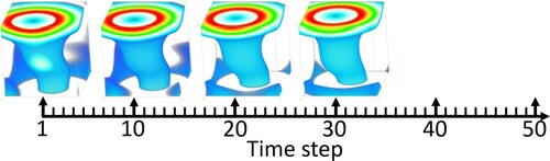Therefore, the essence of the time-varying volumetric data is a four-dimensional matrix $V=p(x,y,z,t)$, where $x,y,z,$ and t are the independent variables; t denotes a specific time step; $(x,y,z)$ denotes the voxel indexed along three spatial directions; p denotes the mapping between a voxel at time step t and its associated value. Figure 1 illustrates the concept of time-varying volumetric data using the Tornado dataset, which depicts the evolution of a tornado over time. From this figure, we can see that this dataset includes a series of tornado volumes spanning 50 time steps. Each time step corresponds to a specific tornado volume. The black axis denotes the time step. In particular, four tornado volumes located at time steps 1, 10, 20, and 30 are being visualised. As for videos, they have a similar concept to time-varying volumetric data, except that they are essentially represented as a 3D matrix $V=q(x,y,t)$, where $x,y,$ and t are the independent variables; t denotes a specific frame in time; $(x,y)$ denotes a pixel indexed along two spatial directions on that frame; q denotes the mapping between a pixel on a frame and its associated value. Although videos and volumetric data have different definitions and independent variables (videos involve both space and time, while volumetric data only involve space), they are both represented as 3D matrices.

Figure 1. The illustration of concept of time-varying volumetric data by using the Tornado dataset, which is visualised at four time steps $1,10,20$, and 30. The black axis denotes the time step.

Given a low-resolution volumetric sequence $V^L=\{v_1^l,v_2^l,\dots ,v_n^l\}$, where $v_i^l$ denotes a single low-resolution volumetric data at the ith time step, our objective is to construct the SSR-DoubleUNetGAN model that can perform the mapping $V^H=M\left(V^L\right)$, where $V^H=\{v_1^h,v_2^h,\dots ,v_n^h\}$ denotes a high-resolution volumetric sequence, and $v_i^h$ denotes the single high-resolution volumetric data at the ith time step corresponding to $v_i^l$.

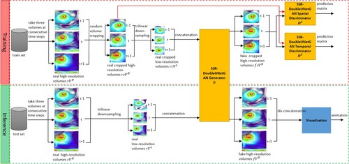
Figure 2 shows the overall framework of our research, which comprises a training stage and an inference stage. During the training stage, we first take three volumes at consecutive time steps from the train set to obtain the real high-resolution volumes $r{V}^H$. Secondly, to increase the amount of training data, we crop $r{V}^H$ at a random position each time to generate the real cropped high-resolution volumes $rc{V}^H$. Third, we apply trilinear down-sampling to $rc{V}^H$ to obtain the real cropped low-resolution volumes $rc{V}^L$. Fourthly, we concatenate the three consecutive volumes in $rc{V}^L$ along the channel dimension and input them into the generator of SSR-DoubleUNetGAN to output the fake cropped high-resolution volumes $fc{V}^H$. Fifth, we input both $fc{V}^H$ and $rc{V}^H$ to the spatial discriminator and temporal discriminator of SSR-DoubleUNetGAN, respectively, to generate the corresponding prediction matrices, which indicate the likelihood of each region of the input being true or false. These steps are repeated for a fixed number of iterations, and ultimately, we can obtain a reliable generator. During the inference stage, similarly to the first step of the training, we first take three consecutive volumes from the test set to obtain the real high-resolution volumes $r{V}^H$. Secondly, we apply trilinear down-sampling to $r{V}^H$ to obtain the real low-resolution volumes $r{V}^L$. Third, we concatenate the three volumes in $r{V}^L$ and input them into the trained generator to synthesise the fake high-resolution volumes $f{V}^H$. Fourthly, we dis-concatenate the three volumes in the inferred $f{V}^H$ and input them into the visualisation module to generate the final animation.

Figure 2. The research framework.

4. SSR-DoubleUNetGAN

As illustrated in Figure 2, our SSR-DoubleUNetGAN consists of a generator, a spatial discriminator, and a temporal discriminator. The generator's job is to take both the spatial coherence and temporal coherence of the time-varying volumetric data into account and try to generate fake high-resolution volumes that are as true as possible, while fooling the discriminators. The role of the spatial discriminator is to guarantee that the spatial differences between the fake and real high-resolution volumes are as small as possible, while the temporal discriminator's job is to guarantee that their temporal differences are as small as possible.

4.1. Network architectures

4.1.1. Generator architecture

Figure 3(a) shows all the operations involved in our generator and discriminators, while Figure 3(b) illustrates the architecture of the generator. As illustrated by the figure, the generator consists of a top (UNet 2) and a bottom (UNet 1) UNet network, and each UNet network has an encoder and a decoder to transform the feature maps. More specifically, the encoder1 contains two Trilinear Upsample (which either upsamples or downsamples a single volume in three spatial x, y, and z directions by using trilinear interpolation, depending on the specified scale factor. If the scale factor is $>1$, then an upsampling occurs; if it is $<1$, then a downsampling occurs)$+1\times 1\times 1$ Conv+Spectral Norm operations that are used to enlarge the low-resolution input, and two Transform Block (TB)+Trilinear Upsample operations that are used to contract the feature maps. In comparison, the encoder2 only contains four TB+Trilinear Upsample operations for contracting the feature maps. Both decoder1 and decoder2 are the same, and they both contain two Transform Block & Self-Attention Block (TB&SAB) and two TB+Trilinear Upsample operations. In addition, we use a TB&SAB to link the encoder and decoder in UNet 1 and UNet 2, respectively. Also, we add UNet 1's output with the volumetric data with dimensions of 128×128×128×3 in it and use this result as input for UNet 2. One thing that deserves special mentioning is that GANs are sometimes prone to checkerboard artefacts or blur as a result of using deconvolution. Therefore, to avoid this issue, we use trilinear upsampling instead in our research.

Figure 3. The SSR-DoubleUNetGAN's generator architecture. (a) The schematic diagram of operations. (b) The generator architecture. (c) The Transform Block (TB). (d) The Transform Block & Self-Attention Block (TB&SAB). (e)The Self-Attention Block (SAB).

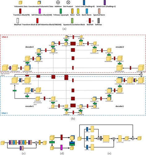
The core of the generator relies on TB, SAB, TB&SAB, and ResPath, as illustrated in Figure 3(a,c,d,e). They all work together to ensure that the generator generates realistic super-resolution volumes. For TB, it has two learning paths: the first path is composed of three convolutions, while the second path consists of one convolution. Finally, the feature maps learned from these two paths are added together and pass through a ReLU activation. Such a design allows the generator to effectively learn different features through separate paths, while also facilitating easier gradient propagation during back-propagation. For SAB, it is used as a supplement to the convolution operation. While the convolution operation can only learn features from nearby voxels, the SAB operation allows for learning features from distant voxels and thus can improve the learning ability of the network. For TB&SAB, it also has two learning paths: one path includes a TB, and the other one first applies the Trilinear Upsample to halve the dimensions of the feature maps, and second applies the SAB, as illustrated in Figure 3(e), to further transform them, and third applies the Trilinear Upsample+1$\times 1\times 1$ Conv to double their dimensions and change their number of channels. Finally, the feature maps from these two paths are concatenated together along the channel. For the ResPath, it is an improvement on the traditional skip connection by adding one or more TBs. From the high-resolution feature maps to the low-resolution feature maps in the generator, we add 1, 2, 3, and 4 TBs, respectively, to the ResPath, as illustrated in Figure 3(b). These ResPath can improve the capability of feature extraction of the generator while allowing for easier back-propagation.

4.1.2. Discriminators architecture

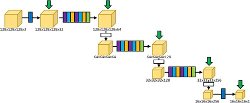
Both the spatial discriminator and temporal discriminator share the same architecture, as shown in Figure 4. It is clear from the figure that the architecture includes two $1\times 1\times 1$ Conv operations at the beginning and end of the network to transform the channel. Furthermore, it contains three consecutive contracting operations in the middle, and each of these operations consists of two $3\times 3\times 3$ Conv operations, followed by a Squeeze & Excitation Block as described in Jha et al. (2019), and a MaxPool operation. We keep this architecture simple because the job of the two discriminators is much easier compared to the job of the generator. In this way, we can ensure a balance between the discriminators and the generator during the training process.

Figure 4. The architecture of the spatial and temporal discriminators.

4.2. Loss functions

4.2.1. Generator loss function

Equation (1(1) $\begin{array}{rl}{\text{Ł}}_G& ={\lambda }^{adv}\times L_G^{adv}+{\lambda }^{spatial}\times L_G^{spatial}+\\ & {\lambda }^{temporal}\times L_G^{temporal}+{\lambda }^{voxdis}\times L_G^{voxdis}\end{array}$(1) ) shows the total loss function of the generator G, which comprises four terms. (1) $\begin{array}{rl}{\text{Ł}}_G& ={\lambda }^{adv}\times L_G^{adv}+{\lambda }^{spatial}\times L_G^{spatial}+\\ & {\lambda }^{temporal}\times L_G^{temporal}+{\lambda }^{voxdis}\times L_G^{voxdis}\end{array}$(1) The first term is the adversarial loss $L_G^{adv}$, as shown in Equation (2(2) $L_G^{adv}=\Vert D^S\left(G\right(rc{V}^L\left)\right)-1{\Vert }_{BCEL}+\Vert D^T\left(G\right(rc{V}^L\left)\right)-1{\Vert }_{BCEL}$(2) ), where $rc{V}^L$ denotes the real cropped low-resolution volumes; $D^S$ and $D^T$ denote the spatial discriminator and temporal discriminator, respectively; $\Vert \cdot {\Vert }_{BCEL}$ denotes the binary cross entropy loss $BCELossWithLogits\left(\right)$. It measures the likelihood that both $D^S$ and $D^T$ consider the fake cropped high-resolution volumes synthesised by the generator to be the ground truth. (2) $L_G^{adv}=\Vert D^S\left(G\right(rc{V}^L\left)\right)-1{\Vert }_{BCEL}+\Vert D^T\left(G\right(rc{V}^L\left)\right)-1{\Vert }_{BCEL}$(2) The second term is the spatial loss $L_G^{spatial}$, as shown in Equation (3(3) $L_G^{spatial}=\frac{1}{5}\times \sum _{n=1}^5\Vert f^n\left(D^S\right(rc{V}^H\left)\right)-f^n\left(D^S\right(G\left(rc{V}^L\right)\left)\right){\Vert }_{MSE}$(3) ), where $rc{V}^H$ denotes the real cropped high-resolution volumes; $f^n$ denotes the feature map at the nth layer (we select 5 feature maps at 5 layers in $D^S$, as illustrated by the green arrows in Figure 4. Therefore, n = 5); $\Vert \cdot {\Vert }_{MSE}$ denotes the MSE loss. It measures the differences between the real feature maps and the fake feature maps in $D^S$. The spatial loss is derived from the feature loss (Han & Wang, 2022a), which serves a similar purpose to the perceptual loss (Wang et al., 2018) and has been shown to be useful for improving GAN training and spatial perceptual quality. (3) $L_G^{spatial}=\frac{1}{5}\times \sum _{n=1}^5\Vert f^n\left(D^S\right(rc{V}^H\left)\right)-f^n\left(D^S\right(G\left(rc{V}^L\right)\left)\right){\Vert }_{MSE}$(3) The third term is the temporal loss $L_G^{temporal}$, as illustrated in Equation (4(4) $\begin{array}{rl}{L}_G^{temporal}& =\frac{1}{4}\times \sum _{n=1}^4\Vert \left[f_{2:L^n}^n\right(D^T\left(rc{V}^H\right))-f_{1:L^n-1}^n(D^T\left(rc{V}^H\right)\left)\right]-\\ & \left[f_{2:L^n}^n\right(D^T\left(G\right(rc{V}^L\left)\right))-f_{1:L^n-1}^n(D^T\left(G\right(rc{V}^L\left)\right)\left)\right]{\Vert }_{MSE}\end{array}$(4) ), where $L^n$ denotes the total number of channel for $f^n$; $f_{2:L^n}^n$ denotes from the second channel to the last channel of $f^n$; $f_{1:L^n-1}^n$ denotes from the first channel to the second last channel of $f^n$. Due to the fact that the last feature map (which is the output of $D^T$) only has one channel and we cannot compute its channel differences, we set n = 4. This term essentially quantifies the disparity between the channel differences of the real feature maps and the fake feature maps. This is a novel loss function invented by us, inspired by the above-mentioned spatial loss. Its principle is explained as follows: as shown in Figure 2, since we concatenate three volumes at three consecutive time steps along the channel, it can be considered as the “time” dimension. Therefore, we hope that the discrepancy between any two channels of the fake feature map is as close as possible to the difference between the corresponding two channels of the real feature map. In this way, we can encourage the synthesised super-resolution volumes to have similar temporal coherence as the ground truth. (4) $\begin{array}{rl}{L}_G^{temporal}& =\frac{1}{4}\times \sum _{n=1}^4\Vert \left[f_{2:L^n}^n\right(D^T\left(rc{V}^H\right))-f_{1:L^n-1}^n(D^T\left(rc{V}^H\right)\left)\right]-\\ & \left[f_{2:L^n}^n\right(D^T\left(G\right(rc{V}^L\left)\right))-f_{1:L^n-1}^n(D^T\left(G\right(rc{V}^L\left)\right)\left)\right]{\Vert }_{MSE}\end{array}$(4) The fourth term is the voxel distance loss, as shown in Equation (5(5) $L_G^{voxdis}=\Vert G\left(rc{V}^L\right)-rc{V}^H{\Vert }_{L1}$(5) ), where $\Vert \cdot {\Vert }_{L}1$ denotes the $L1$ loss. It measures the voxel distance between the real cropped high-resolution volumes and the fake cropped high-resolution volumes generated by the generator. ${\lambda }^{adv},{\lambda }^{spatial},{\lambda }^{temporal}$ and ${\lambda }^{voxdis}$ denote the weights for the above-mentioned terms. (5) $L_G^{voxdis}=\Vert G\left(rc{V}^L\right)-rc{V}^H{\Vert }_{L1}$(5)

4.2.2. Discriminators' loss function

Equation (6(6) $L_{D^S}=\frac{1}{2}\times (\Vert D^S(G\left(rc{V}^L\right))-0{\Vert }_{BCEL}+\Vert D^S(rc{V}^H)-1{\Vert }_{BCEL})$(6) ) shows the loss function of $D^S$, which consists of two terms. The first term measures the likelihood of $D^S$ determining the fake cropped high-resolution volumes generated by the generator to be false, while the second term measures the likelihood of $D^S$ determining the real cropped high-resolution volumes to be true. We calculate the average of them and use it as the final loss. (6) $L_{D^S}=\frac{1}{2}\times (\Vert D^S(G\left(rc{V}^L\right))-0{\Vert }_{BCEL}+\Vert D^S(rc{V}^H)-1{\Vert }_{BCEL})$(6) Equation (7(7) $L_{D^T}=\frac{1}{2}\times (\Vert D^T(G\left(rc{V}^L\right))-0{\Vert }_{BCEL}+\Vert D^T(rc{V}^H)-1{\Vert }_{BCEL})$(7) ) shows the loss function of $D^T$, which contains two similar terms as in Equation (6(6) $L_{D^S}=\frac{1}{2}\times (\Vert D^S(G\left(rc{V}^L\right))-0{\Vert }_{BCEL}+\Vert D^S(rc{V}^H)-1{\Vert }_{BCEL})$(6) ). (7) $L_{D^T}=\frac{1}{2}\times (\Vert D^T(G\left(rc{V}^L\right))-0{\Vert }_{BCEL}+\Vert D^T(rc{V}^H)-1{\Vert }_{BCEL})$(7)

4.3. Training stability improvement

We utilise three techniques to enhance the training stability of our model. The first technique is the Two Timescale Update Rule (TTUR) (Zhang et al., 2019), which uses different learning rates for the generator and discriminator, allowing for fewer updates to the discriminator per generator update. The second technique is Spectral Normalisation (Miyato et al., 2018) (abbreviated as Spectral Norm in our research), which is a weight normalisation approach that offers several advantages. One advantage (Lin et al., 2021) is that it can mitigate exploding gradients by limiting the ability of weight tensors to amplify inputs in any direction. Additionally, it can mitigate the issue of vanishing gradients during training. Since both issues are closely related to the instability of GANs, addressing them can ultimately enhance the training stability of GANs. Another advantage is that, unlike other normalisation techniques that require additional hyperparameters, it only needs to be set after the convolution operation without any additional hyperparameter. A third advantage is that it can save computational costs during training. The third technique is the Self-attention mechanism (Zhang et al., 2019). In comparison to the traditional convolution operation, which only learns features from nearby voxels, it can learn features from distant voxels, thereby enhancing the network's learning ability.

5. Visualisation

We use the volume ray casting algorithm in conjunction with the jet colourmap to generate all visualisation results. We render each volume at a time step as a single frame, allowing us to create an animation of the entire time-varying volumetric data. Moreover, in order to clearly reveal the difference between the synthesised super-resolution from different techniques and the ground truth, we compute their difference and show the corresponding visualisation results.

6. Implementation

For our model, we utilise the PyTorch library for implementation and train/infer it on a Dell server equipped with an NVIDIA GTX 3090 GPU that has 24GB video memory. For visualisation, we use CUDA and OpenGL/GLUT to implement it and render its results on a local desktop computer that has an NVIDIA GTX 1060 GPU with 6GB video memory. For each dataset used in the research, we use its first 70% for the training and the remaining 30% for the inference. We set batch size = 1; ${\lambda }^{adv}=1$; ${\lambda }^{spatial}=1$; ${\lambda }^{temporal}=1$; ${\lambda }^{voxdis}=1$; the generator's learning rate = 0.0002; the spatial and temporal discriminators' learning rate = 0.00002; the number of updates per batch for the generator, the spatial discriminator, and the temporal discriminator are 1, 1, 1, respectively. The number of epochs used for training and the scale factor used for super-resolution generation for each dataset are listed in Table 1.

Table 1. The name, dimensions, scaling factor, number of epochs for training, consumed training time and inference time of each dataset.

Dataset	Dimensions($x\times y\times z\times t$)	Scaling factor	Number of epochs	Training time (s)	Inference time (s)
SquareCylinder	192 × 64 × 48 × 102	4	20	651.18	3.19
Hurricane (wind)	250 × 250 × 50 × 48	5	50	1065.46	4.63
Hurricane (QSNOW)	250 × 250 × 50 × 48	5	15	314.97	–
Hurricane (QICE)	250 × 250 × 50 × 48	5	–	–	4.35
ViscousFingers	100 × 100 × 100 × 121	5	12	497.02	4.75
Ionisation (H)	150 × 100 × 100 × 100	5	40	1259.76	4.91

7. Results and discussion

This section presents and discusses our experimental results. In addition to the Ground Truth and our method, five comparison methods have been carefully selected for the research. The first method is SSR-TVD (Han & Wang, 2022a), which is the most recent state-of-the-art super-resolution technique for time-varying volumetric data. The second method is SRResNet (Ledig et al., 2017), which is a classic super-resolution technique for a single image, and we extend and apply it to time-varying volumetric data. Specifically, we modify 2D convolution, pixel shuffle, and normalisation in the original version to be 3D convolution, pixel shuffle, and normalisation so that it can process volumes rather than images. The third is the Tricubic technique (Lekien & Marsden, 2005), which is a 3D version of Bicubic interpolation that is often used as a comparison method for the super-resolution research on 2D images. The fourth and fifth methods are the Cubic and Linear techniques, which are widely known interpolation baselines.

To ensure a fair comparison between our method and the SSR-TVD and SRResNet deep learning models mentioned above, it is crucial to use the same data for training/inference. This includes using the same low-resolution input and high-resolution output. Also, they are run on the same hardware, which is the NVIDIA GTX 3090 GPU as mentioned in Section 6. As we adhere to the parameters e.g. normalisation, upsampling or downsampling schemes, etc., proposed in the original SSR-TVD and SRResNet, they may vary among these deep learning models. In addition, the hyperparameters used in these deep learning models could vary because they are distinct models with different characteristics e.g. some models may have a faster learning ability, while others may have a slower learning ability. But for each deep learning model, we have tried our best to fine-tune its hyperparameters to generate the best super-resolution results.

To demonstrate their effectiveness, we applied several time-varying volumetric datasets from various simulations to them. We also compared their similarities in synthesising super-resolution with respect to the Ground Truth, both qualitatively and quantitatively. Furthermore, we conducted an ablation study to assess the validity of the core modules in our model.

7.1. Qualitative analysis

7.1.1. Training and inference with the same variable

This section introduces the visualisation results of the synthesised super-resolution time-varying volumetric data that are obtained by using the same variable of a dataset for both training and inference.

7.1.1.1 SquareCylinder dataset

This dataset is a 3D time-dependent incompressible flow field with a Reynolds number of 200 and the square cylinder has been positioned symmetrically between two parallel walls. It was obtained from a direct numerical Navier-Stokes simulation conducted by Cammarri et al. (2005) which is publicly available (International CFD database, n.d.). We use a uniformly resampled version which has been provided by Tino Weinkauf and used in von Funck et al. for smoke visualisation (Funck et al., 2008).

Figure 5 shows the visualisation results of the SquareCylinder dataset at four time steps from the Ground Truth, our method, SSR-TVD, Tricubic, SRResNet, Cubic, and Linear. More specifically, each row in the figure represents the visualisation results at different time steps from the same method (the method name is listed on the left), while each column in the figure corresponds to the visualisation results at the same time step (the time step is listed on the top) from different methods. The bottom right smaller image of each figure shows the absolute difference visualisation between the volume on that figure and its corresponding Ground Truth, which allows us to better distinguish their similarity. For each bottom right smaller image, we can utilise opacity and colour rules to determine whether or not it is more similar to the Ground Truth:

• opacity rule: if its visualisation is more transparent, then it is more similar to the Ground Truth; if its visualisation is less transparent, then it is less similar to the Ground Truth.

• colour rule: if its visualisation is more bluish, then it is more similar to the Ground Truth; if its visualisation is more reddish, then it is less similar to the Ground Truth.

Figure 5. The visualisation of the synthesised high-resolution SquareCylinder dataset from (a) the Ground Truth, (b) our method, (c) SSR-TVD, (d) Tricubic, (e) SRResNet, (f) Cubic, and (g) Linear.

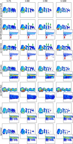
Based on the rules, we can quickly recognise from the bottom right smaller images that both Tricubic and SRResNet generate the least similar super-resolution results to the Ground Truth, as their visualisation is the most opaque (by closely comparing the Tricubic with SRResNet, it is clear that the Tricubic is superior than SRResNet, since the super-resolution data generated from SRResNet is distorted and it is impossible to see the shapes of the flow field). The Cubic and Linear generate the second least similar super-resolution results to the Ground Truth, as their visualisation is the second most opaque. Also, their visualisation shows more reddish. In contrast to the Cubic and Linear, both the visualisation of our method and SSR-TVD are the most transparent, and is more bluish. Therefore, both our method and SSR-TVD can generate the most similar super-resolution results to the Ground Truth. By comparing our method with SSR-TVD, we can conclude that our method is superior in super-resolution synthesis than SSR-TVD for two reasons: firstly, as shown by the red arrows, the big flow field object in our method is more transparent than the one in SSR-TVD; secondly, as indicated by the green arrows, the shapes of the flow field objects in our method are closer to the Ground Truth than those in SSR-TVD.

7.1.1.2 ViscousFingers dataset

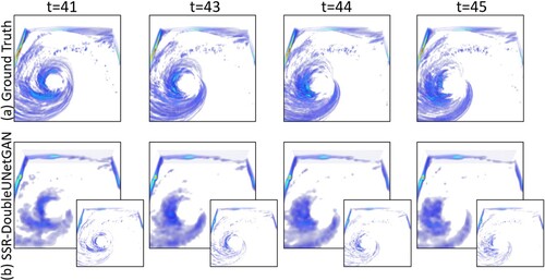
This dataset is generated from the finite pointset method (FPM)-based simulations, which simulate the behaviour of salt dissolving in water and generate several ensembles of particle data at three different resolution levels (known as the smooth length). During the process of simulations, viscous fingers emerge, which are areas within the cylinder volume with increased salt concentration (Aldrich et al., 2016). We employ the dataset from the first ensemble member (run01) with a smooth length of 0.30 for our research, and convert it from particle data to regular grid-based volume data using a preprocess similar to Aldrich et al. (2016).

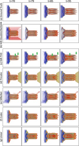
Figure 6 shows the visualisation results of the ViscousFingers dataset at four time steps from the Ground Truth, our method, SSR-TVD, Tricubic, SRResNet, Cubic, and Linear. Again, each row in the figure represents the visualisation results at different time steps from the same method, while each column corresponds to the visualisation results at the same time step from different methods. The bottom left smaller image of each figure shows the absolute difference visualisation between the volume on that figure and its corresponding Ground Truth.

Figure 6. The visualisation of the synthesised high-resolution ViscousFingers dataset from (a) the Ground Truth, (b) our method, (c) SSR-TVD, (d) Tricubic, (e) SRResNet, (f) Cubic, and (g) Linear.

According to the above-mentioned opacity and colour rules it is clear from the bottom left smaller images that our method has the most transparent visualisation results e.g. at those areas indicated by the green arrows, and thus it can generate the closest results to the Ground Truth. The SRResNet appears to produce the second most transparent visualisation results, leading us to consider it as the second best method. On the contrary, the Tricubic has the least transparent visualisation results, and thus it is the worst in super-resolution synthesis. For the remaining three techniques, namely SSR-TVD, Cubic, and Linear, it appears that their visualisation have similar opacity and colour. However, upon further comparison of the areas indicated by the red arrows, it is evident that the visualisation results from the Cubic technique preserve more details than those from the SSR-TVD and Linear techniques.

7.1.1.3 Hurricane (wind) dataset

The dataset is a simulation of hurricane named Isabel generated by the Weather Research and Forecast (WRF) model developed by the National Center for Atmospheric Research in the United States. The dataset consists of several time-varying scalar and vector variables with large dynamic ranges.

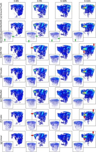
Figure 7 shows the visualisation results of the Hurricane (wind) dataset at four time steps from the Ground Truth, our method, SSR-TVD, Tricubic, SRResNet, Cubic, and Linear. The upper right smaller image of each figure shows the absolute difference visualisation between the volume on that figure and its corresponding Ground Truth.

Figure 7. The visualisation of the synthesised high-resolution Hurricane (wind) dataset from (a) the Ground Truth, (b) our method, (c) SSR-TVD, (d) Tricubic, (e) SRResNet, (f) Cubic, and (g) Linear.

According to the above-mentioned opacity and colour rules we can see from the upper right smaller images that the SRResNet has the least transparent visualisation results, and thus it is the worst method for super-resolution synthesis. Tricubic seems to have the second least transparent visualisation results, and thus it is the second worst method. The remaining four techniques have more transparent visualisation results, which indicate they are better methods for super-resolution synthesis. More specifically, in contrast to the hurricane eyes in our method and SSR-TVD, we can observe that the ones in both Cubic and Linear techniques are less transparent, which indicates that both our method and SSR-TVD are more accurate than Cubic and Linear techniques in synthesising super-resolution volumes. Furthermore, by carefully comparing the visualisation results from our method and from the SSR-TVD, we have discovered that in the areas indicated by the red arrows, our visualisation is more transparent than that of the SSR-TVD. Therefore, our method outperforms SSR-TVD in super-resolution synthesis.

7.1.2 Training and inference with different variables

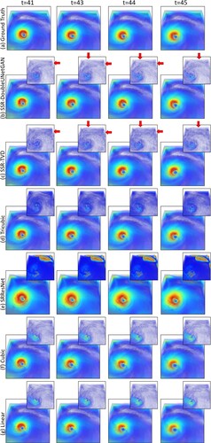
In addition to using the same variable for both training and inference, our method also allows for using one variable from a dataset for training and another variable from the same dataset for inference. Figure 8 shows the visualisation results of the Hurricane (QICE) at four time steps from the Ground Truth and our method. In this case, we first use the Hurricane (QSNOW) variable to train our model, and then apply the trained model to the Hurricane (QICE) variable for inference. The bottom right image of each figure shows the visualisation of the absolute difference between that figure and its corresponding Ground Truth. It is clear from Figure 8 that although the synthesised super-resolution data from our method lose some fine details, they can still approximate the hurricane eye to some extent.

Figure 8. The visualisation of the synthesised high-resolution Hurricane (QICE) from (a) the Ground Truth, (b) our method. In this case, we use the Hurricane (QSNOW) variable to train our model and use the Hurricane (QICE) variable for inference.

7.2. Quantitative analysis

7.2.1. Quantitative metrics

We use three metrics to evaluate our method and the state-of-the-art techniques from two perspectives. Firstly, we use both Peak Signal-to-Noise Ratio (PSNR) and Structural Similarity Index Measure (SSIM) to evaluate the synthesised super-resolution volumes of different methods in reference to the Ground Truth volumes from the “volume” perspective. Secondly, we use the Mean Opinion Scores (MOS) (Han & Wang, 2022a; Ledig et al., 2017) to evaluate the rendered images of the synthesised volumes in reference to the Ground Truth images from the “perception” perspective.

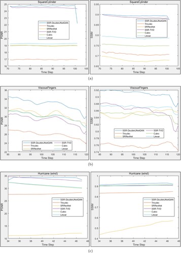
The left figure in Figure 9(a) shows the PSNR comparison of the synthesised time-varying volumes from different methods for the SquareCylinder dataset. From this figure, it is clear that our method is much superior than the Tricubic, SRResNet, Cubic, and Linear techniques (since it has much bigger PSNR values), and is slightly superior than the SSR-TVD except at the beginning and end of the time steps. The right figure in Figure 9(a) shows the SSIM comparison of all methods for the same dataset, and it is clear from the figure that our method also slightly outperforms SSR-TVD, and is far better than the Tricubic, SRResNet, Cubic, and Linear techniques. Figure 9(b) shows the PSNR and SSIM comparison of all methods for the ViscousFingers dataset. From the figure, it is clear that our method outperforms all other methods, while the Tricubic has the worst performance. Figure 9(c) shows the PSNR and SSIM comparison of all methods for the Hurricane (wind) dataset. For the PSNR comparison, it is clear from the figure that our method slightly outperforms SSR-TVD except at the beginning of the time steps, and is much superior than Tricubic, SRResNet, Cubic, and Linear techniques. For the SSIM comparison, our method is slightly better than the SSR-TVD, Cubic, and Linear techniques, and is much superior than both Tricubic and SRResNet techniques.

Figure 9. The PSNR and SSIM comparison of different methods in reference to the Ground Truth volumes for (a) SquareCylinder, (b) ViscousFingers and (c) Hurricane (wind) datasets.

To obtain the MOS comparison of different methods in reference to the Ground Truth, we performed a user study. For each dataset, we show its seven animated visualisation that corresponds to the Ground Truth, our method, SSR-TVD, Tricubic, SRResNet, Cubic, and Linear, respectively, side by side. The animated visualisation can be played frame by frame by pressing the “space” key on the keyboard. Also, we enable mouse functionalities including zooming in/out, rotation, translation for the animated visualisation so that the user can better observe the visualisation results. A total of 15 master students from school of computer science in our university have been recruited for the user study. After providing a brief introduction to the research context and goals, we asked each student to evaluate how closely the visualisation results of the synthesised super-resolution from different methods are with respect to the visualisation of the Ground Truth by assigning a score ranging from 1 (least similar) to 10 (most similar). Table 2 shows the MOS values. It is clear from the table that our method has the biggest MOS values for all datasets, which indicate it is the best method for super-resolution synthesis. On the contrary, SRResNet has the smallest values for all datasets, which indicate it is the worst method. The main reason for this is because the visualisation results of SRResNet have the Checkerboard Artifacts.

Table 2. The MOS comparison of all methods for each dataset.

Dataset	Our method	SSR-TVD	Tricubic	SRResNet	Cubic	Linear
SquareCylinder	7.8	6.9	7.5	4.2	7.0	7.4
Hurricane (wind)	8.8	8.0	6.8	5.6	7.1	7.5
ViscousFingers	8.3	7.4	8.0	7.1	8.0	7.5

Note: The best scores are indicated in bold.

7.3. Performance

Table 1 shows the performance of our model. It is clear from the table that our model requires only a very small number of epochs and a very short training and inference time for each dataset to achieve good synthesis results. This is significantly better than some state-of-the-art techniques e.g. SSR-TVD (Han & Wang, 2022a) that require a large number of epochs and a significant amount of time for training. Table 3 shows the performance of our visualisation. It is clear that the SquareCylinder dataset has the fastest FPS, while the ViscousFingers has the slowest FPS.

Table 3. The Frames Per Second (FPS) of our visualisation for each dataset.

Dataset	FPS
SquareCylinder	24
Hurricane (wind)	16
ViscousFingers	9

7.4. Ablation study

To test the validity of the core modules in our model, we conducted an ablation study using the Hurricane (wind) dataset. The study involved six variants of our model, as listed in Table 4. For each variant model, it only contains one modified module compared to our model. More specifically, Model_TBwithoutRes represents a model where the residual paths of all TB operations are removed. Model_Conv4TB represents the model where we use $3\times 3\times 3$ convolution operations to replace all TB operations. Model_NoSAB represents the model where we remove all SAB operations. Model_ResBlocks4Bridges denotes the model where we use 7 residual blocks to replace a $TB\mathrm{\&}SAB$ operation for any bridge that links a pair of encoder and decoder. Model_SkipCon4ResPath denotes the model where we use skip connection to replace the ResPath. Finally, Model_Multiply4Add denotes the model where we use the multiplication operation to replace the addition operation, as shown in Figure 3(b).

Table 4. The ablation study of our model.

Model Name	TB	TB&SAB (in encoders/decoders)	TB&SAB (as bridges)	ResPath	Addition
Our method	✓	✓	✓	✓	✓
Model_TBwithoutRes	TB without Residual	TB without Residual&SAB	TB without Residual&SAB	TB without Residual-based ResPath	✓
Model_Conv4TB	Conv	Conv&SAB	Conv&SAB	Conv-based ResPath	✓
Model_NoSAB	✓	TB	TB	✓	✓
Model_ResBlocks4Bridges	✓	✓	Residual Blocks	✓	✓
Model_SkipCon4ResPath	✓	✓	✓	Skip Connection	✓
Model_Multiple4Add	✓	✓	✓	✓	Multiply4Add

Note: For each variant model, only one module is changed.

Figure 10 shows the PSNR and SSIM values of all models involved in the ablation study in reference to the Ground Truth. For the PSNR values, it is clear from the figure that our model outperforms all variants except for the first and last time steps. For the SSIM values, we also can observe that our model outperforms all variants except at the last time step. Through the ablation study, we prove that the combination of the modules in our current model is optimised, in comparison to its variants. We further analyse the rationale behind this as follows: in comparison to Model_Conv4TB, the reason why our model is more accurate is because our TB module is superior than the pure convolution operations in capturing feature details. Compare to Model_Multiply4Add, the reason why our model is more accurate is because the addition operation can better combine two feature maps together than the multiplication operation. Compared to Model_NoSAB, the reason why our model is more accurate is because our SAB module allows to learn features from distant voxels and thus can enhance the learning ability of the network. Compared to Model_ResBlocks4Bridges, the reason why our model is more accurate is because the $TB\mathrm{\&}SAB$ module is superior than the residual blocks in transforming the features between the encoder and decoder. Compared to Model_SkipCon4ResPath, the reason why our model is more accurate is because ResPath can better transform the encoder's features to the decoder's features, and thus is superior than the skip connection. Finally, in comparison to Model_TBwithoutRes, the reason why our model is more accurate is because by adding the residual paths, our TB module allows the network to learn different features via different paths and thus is superior than the TB module without residual paths.

Figure 10. The PSNR and SSIM values for different models involved in the ablation study of our model.

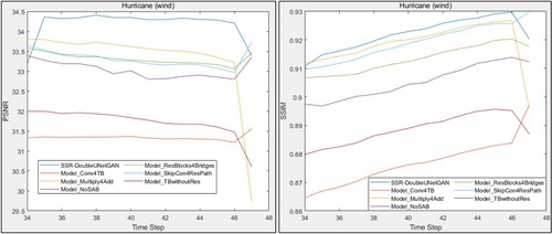
Figure 11. The visualisation of the synthesised high-resolution Ionisation (H) from (a) the Ground Truth, (b) our method, (c) SSR-TVD, (d) Tricubic, (e) SRResNet, (f) Cubic, and (g) Linear.

7.5. Limitations

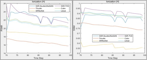
Our method does not always outperform the state-of-the-art techniques, and one example of this is the Ionisation (H) dataset. Figure 11 shows the visualisation results of the synthesised Ionisation (H) from the Ground Truth and all compared methods. It is evident from the figure that SSR-TVD outperforms our method in preserving the fine details of the data e.g. at the top and interior, as indicated by the green arrows. Figure 12 shows both PSNR and SSIM values of all methods for the Ionisation (H) dataset. It is evident that our method slightly outperforms SSR-TVD in terms of PSNR, except at the beginning of the time steps. However, our method performs worse than SSR-TVD, Cubic, and Linear techniques when evaluated using SSIM.

Figure 12. The PSNR and SSIM comparison of all methods inference to the Ground Truth for the Ionisation (H) dataset.

7.6. Discussion

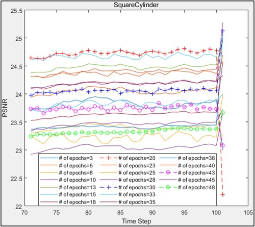
As shown in the left image of Figure 9(a), there is a sudden decline in the PSNR at the end of the time steps for the SquareCylinder dataset. To determine the possible cause of this behaviour, we saved multiple super-resolution synthesis results from our model across multiple number of epochs for the SquareCylinder dataset, and plot their PSNR, as demonstrated in Figure 13. From this figure, we can see that sometimes the PSNR declines at the end of time steps e.g. as illustrated by the red and magenta lines, and sometimes it goes up e.g. as indicated by the blue and green lines. Therefore, we attribute this behaviour to the randomness of our model.

Figure 13. The PSNR values of the synthesised super-resolution volumes from our model at multiple number of epochs for the SquareCylinder dataset.

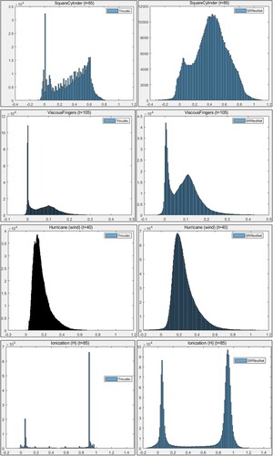
As shown in Figures 9 and 12, the Tricubic is worse than the SRResNet in PSNR for all except the Hurricane (wind) dataset. To find out the possible reason, we sample the synthesised super-resolution volumes at a random time step from the Tricubic and SRResNet for all datasets and plot their histograms, as demonstrated in Figure 14. From the figure, we can see that only the Hurricane (wind) dataset has a unimodal-like data distribution, while all other datasets have bimodal-like data distribution. Therefore, we guess that the performance of the Tricubic and SRResNet techniques is dependent on the unimodal or bimodal data distribution.

Figure 14. The data distribution of the synthesised super-resolution volumes at a random time step (as listed in each figure's title) from the Tricubic (left) and SRResNet (right) techniques for all datasets.

8. Conclusions and future works

This paper introduces SSR-DoubleUNetGAN, a GAN-based technique that can accurately and quickly synthesise spatial super-resolution for time-varying volumetric data. It contains three main components: the generator, the spatial discriminator, and the temporal discriminator. The generator consists of two stacked UNet networks, with the goal of generating super-resolution volumes that closely resemble the Ground Truth. The goals of the spatial and temporal discriminators are to distinguish the synthesised volumes from the perspectives of space and time, respectively. We applied several time-varying volumetric datasets from various scientific simulations to our method to demonstrate its effectiveness. We also compared it qualitatively and quantitatively with state-of-the-art techniques. Additionally, we conducted an ablation study to assess the validity of the key modules in our model. The experimental results show that, in most cases, our method can generate more accurate super-resolution time-varying volumes than the state-of-the-art techniques with a short training time.

We expect to do three future works. Firstly, considering the current popularity of the diffusion model, we plan to utilise it for synthesising the spatial super-resolution of time-varying volumetric data. Secondly, our current work is focused solely on the “spatial” super-resolution of time-varying volumetric data. In the future, we would also like to synthesise “temporal” or even “spatio-temporal” super-resolution of time-varying volumetric data. Thirdly, our current work is only focused on synthesising scalar data. In the future, we would also like to perform variable-to-variable or scalar-to-vector (Gu et al., 2022) translation of time-varying volumetric data.

Disclosure statement

No potential conflict of interest was reported by the author(s).

Data availability statement

The data that support the findings of this study are openly available in IEEE SciVis Contest repository at https://sciviscontest.ieeevis.org/.

Additional information

Funding

This work was funded by the Natural Science Foundation of Zhejiang Province of China [grant number LTGY23F020007], and by the Humanities and Social Sciences Foundation of Ministry of Education of China [grant number 23YJC760011].

References

- Aldrich, G., Lukasczyk, J., Steptoe, M., Maciejewski, R., Leitte, H., & Hamann, B. (2016). Viscous fingers: A topological visual analytic approach. In IEEE visualization 2016 scientific visualization contest. Baltimore, Maryland.
- Bai, Z. H., Tao, Y. B., & Lin, H. (2020). Time-varying volume visualization a survey. Journal of Visualization, 23(5), 745–761. https://doi.org/10.1007/s12650-020-00654-x
- Begin, I., & Ferrie, F. P. (2007). PSF recovery from examples for blind super-resolution. In IEEE International conference on image processing (pp. 421–424). San Antonio, TX, USA.
- Blattmann, A., Rombach, R., Ling, H., Dockhorn, T., Kim, S. W., Fidler, S., & Kreis, K. (2023). Align your latents: High-Resolution video synthesis with latent diffusion models. In IEEE/CVF conference on computer vision and pattern recognition (CVPR) (pp. 22563–22575). Vancouver Canada.
- Cammarri, S., Salvetti, M. V., Buffoni, M., & Iollo, A. (2005). Simulation of the three-dimensional flow around a square cylinder between parallel walls at moderate Reynolds numbers. In XVII congresso di meccanica teorica ed applicata.
- Chen, J. N., Lu, Y. Y., Yu, Q. H., Luo, X. D., Adeli, E., Wang, Y., & Zhou, Y. Y. (2021). TransUNet: Transformers make strong encoders for medical image segmentation. arXiv.
- Chen, N. X., Zhang, Y., Zen, H. G., Weiss, R. J., Norouzi, M., & Chan, W. (2021). WaveGrad estimating gradients for waveform generation. In Proc. of international conference on learning representations (ICLR). Vienna, Austria.
- Cicek, O., Abdulkadir, A., Lienkamp, S. S., Brox, T., & Ronnerberger, O. (2016). 3D U-Net: Learning dense volumetric segmentation from sparse annotation. In Medical image computing and computer-assisted intervention (MICCAI) (pp. 424–432). Springer International Publishing.
- Ding, Y., Zhang, C., Cao, M. S., Wang, Y. L., Chen, D. J., Zhang, N., & Z. G. Qin (2021). ToStaGAN: An end-to-end two-stage generative adversarial network for brain tumor segmentation. Neurocomputing, 462, 141–153. https://doi.org/10.1016/j.neucom.2021.07.066
- Funck, W. V., Weinkauf, T., Theisel, H., & Seidel, H. P. (2008). Smoke surfaces: An interactive flow visualization technique inspired by real-World flow experiments. IEEE Transactions on Visualization and Computer Graphics (Proceedings Visualization 2008), 14(6), 1396–1403. https://doi.org/10.1109/TVCG.2008.163http://tinoweinkauf.net/.
- Gong, C. W., Jing, C. H., Chen, X. H., Pun, C. M., Huang, G. L., Saha, A., & Wang, S. Q. (2023). Generative AI for brain image computing and brain network computing: A review. Frontiers in Neuroscience, 17, 1203104. https://doi.org/10.3389/fnins.2023.1203104
- Greenspan, H. (2008). Super-resolution in medical imaging. The Computer Journal, 52(1), 43–63. https://doi.org/10.1093/comjnl/bxm075
- Gu, P. F., Han, J., Chen, D. Z., & Wang, C. L. (2022). Scalar2Vec: Translating scalar fields to vector fields via deep learning. In IEEE 15th pacific visualization symposium (pacificVis). Tsukuba, Japan.
- Gu, Y. C., Zeng, Z. T., Chen, H. B., Wei, J., Zhang, Y. Q., Chen, B. H., & Lu, Y. (2020). MedSRGAN: Medical images super-resolution using generative adversarial networks. Multimedia Tools and Applications, 79(29-30), 21815–21840. https://doi.org/10.1007/s11042-020-08980-w
- Guan, S., Khan, A. A., Sikdar, S., & Chitnis, P. V. (2019). Fully dense UNet for 2d dparse photoacoustic tomography artifact removal. IEEE Journal of Biomedical and Health Informatics, 24(2), 568–576. https://doi.org/10.1109/JBHI.6221020
- Guo, L., Ye, S. J., Han, J., Zheng, H., Guo, H., Chen, D. Z., & Wang, C. L. (2020). SSR-VFD: Spatial super-resolution for vector field data analysis and visualization. In IEEE pacific visualization symposium. Tianjin, China.
- Han, J., & Wang, C. L. (2020). TSR-TVD: Temporal super-resolution for time-varying data analysis and visualization. IEEE Transactions on Visualization and Computer Graphics, 26(1), 205–215.
- Han, J., & Wang, C. L. (2022a). SSR-TVD: Spatial super-resolution for time-varying data analysis and visualization. IEEE Transactions on Visualization and Computer Graphics, 28(6), 2445–2456.
- Han, J., & Wang, C. L. (2022b). TSR-VFD: Generating temporal super-resolution for unsteady vector field data. Computers and Graphics, 103, 168–179. https://doi.org/10.1016/j.cag.2022.02.001
- Han, J., Zheng, H., Chen, D. Z., & Wang, C. L. (2022). STNet: An end-to-end generative framework for synthesizing spatiotemporal super-resolution volumes. IEEE Transactions on Visualization and Computer Graphics, 28(1), 270–280. https://doi.org/10.1109/TVCG.2021.3114815
- Ho, J., Saharia, C., Chan, W., Fleet, D. J., Norouzi, M., & Salimans, T. (2022). Cascaded diffusion models for high fidelity image generation. The Journal of Machine Learning Research, 23(1), 2249–2281.
- Hu, M. S., Jiang, K., Liao, L., Xiao, J., Jiang, J. J., & Wang, Z. (2022). Spatial-Temporal space hand-in-hand: Spatial-Temporal video super-resolution via cycle-projected mutual learning. In IEEE/CVF conference on computer vision and pattern recognition (CVPR). New Orleans, Louisiana.
- Hu, S. Y., Lei, B. Y., Wang, S. Q., Wang, Y., Feng, Z. G., & Shen, Y. Y. (2022). Bidirectional mapping generative adversarial networks for brain MR to PET synthesis. IEEE Transactions on Medical Imaging, 41(1), 145–157. https://doi.org/10.1109/TMI.2021.3107013
- Huang, H. M., Lin, L. F., Tong, R. F., Hu, H. J., Zhang, Q. W., Iwamoto, Y., & Wu, J. (2020). UNet+: 3 a full-scale connected UNet for medical image segmentation Unet 3+: a full-scale connected unet for medical image segmentation. In IEEE international conference on acoustics, speech and signal processing (ICASSP).
- Huang, Y. W., Shao, L., & Frangi, A. F. (2017). Simultaneous super-resolution and cross-modality synthesis of 3d medical images using weakly-supervised joint convolutional sparse coding. In IEEE conference on computer vision and pattern recognition (CVPR). Honolulu, HI, USA.
- Ibehaz, N., & Rahman, M. S. (2020). MultiResUNet: Rethinking the U-Net architecture for multimodal biomedical image segmentation. Neural Networks, 121, 74–87. https://doi.org/10.1016/j.neunet.2019.08.025
- Iglovikov, V., & Shvets, A. (2018). TernausNet: U-Net with VGG11 encoder pre-trained on imagenet for image segmentation. arXiv.
- International CFD database (n.d.). 1. http://cfd.cineca.it/.
- Jha, D., Riegler, M. A., Johansen, D., Halvorsen, P., & Johansen, H. D. (2020). DoubleU-Net: A deep convolutional neural network for medical image segmentation. arXiv.
- Jha, D., Smedsrud, P. H., Riegler, M. A., Johansen, D., Lange, T. D., Halvorsen, P., & Johansen, H. D. (2019). ResUNet++: an advanced architecture for medical image segmentation Resunet++: an advanced architecture for medical image segmentation. In IEEE international symposium on multimedia (ISM). Laguna Hills, California.
- Jiang, K., Wang, Z. Y., Yi, P., & Jiang, J. J. (2020). Hierarchical dense recursive network for image super-resolution. Pattern Recognition, 107, 107475. https://doi.org/10.1016/j.patcog.2020.107475
- Jiang, K., Wang, Z. Y., Yi, P., Wang, G. C., Gu, K., & Jiang, J. J. (2019). ATMFN: Adaptive-Threshold-Based multi-model fusion network for compressed face Hallucination. IEEE Transactions on Multimedia, 22(10), 2734–2747. https://doi.org/10.1109/TMM.6046
- Jiang, K., Wang, Z. Y., Yi, P., Wang, G. C., Lu, T., & Jiang, J. J. (2019). Edge-Enhanced GAN for remote sensing image superresolution. IEEE Transactions on Geoscience and Remote Sensing, 57(8), 5799–5812. https://doi.org/10.1109/TGRS.36
- Jo, Y., Oh, S., Kang, J., & Kim, S. J. (2018). Deep video super-resolution network using dynamic upsampling filters without explicit motion compensation. In IEEE/CVF conference on computer vision and pattern recognition (CVPR). Salt Lake city, UT, USA.
- Kim, B., Han, I., & Ye, J. C. (2022). DiffuseMorph: Unsupervised deformable image registration Using diffusion model. In European conference on computer vision (pp. 347–364). Tel Aviv, Israel.
- Kong, L., Lian, C., Huang, D., Hu, Y., & Zhou, Q. (2021). Breaking the dilemma of medical image-to-image translation. Advances in Neural Information Processing Systems, 34, 1964–1978.
- Lai, W. S., Huang, J. B., Ahuja, N., & Yang, M. H. (2017). Deep laplacian pyramid networks for fast and accurate superresolution. In Proceedings of the IEEE conference on computer vision and pattern recognition (pp. 624–632). Honolulu, HI, USA.
- Ledig, C., Theis, L., Huszar, F., Caballero, J., Cunningham, A., Acosta, A., & Shi, W. (2017). Photo-realistic single image super-resolution using a generative adversarial network. In Proceedings of ieee conference on computer vision and pattern recognition (pp. 4681–4690). Honolulu, HI, USA.
- Lekien, F., & Marsden, J. (2005). Tricubic interpolation in three dimensions. International Journal for Numerical Methods in Engineering, 63(3), 455–471. https://doi.org/10.1002/(ISSN)1097-0207
- Lepcha, D. C., Goyal, B., Dogra, A., & Goyal, V. (2023). Image super-resolution: A comprehensive review, recent trends, challenges and applications. Information Fusion, 91, 230–260. https://doi.org/10.1016/j.inffus.2022.10.007
- Li, S., He, F. X., Du, B., Zhang, L. F., Xu, Y. H., & Tao, D. C. (2019). Fast spatio-remporal residual network for video super-resolution. In IEEE/CVF conference on computer vision and pattern recognition (CVPR). Long Beach, CA, USA.
- Li, Z., Yang, J. L., Liu, Z., Yang, X. M., Jeon, G., & Wu, W. (2019). Feedback network for image super-resolution. In IEEE/CVF conference on computer vision and pattern recognition (CVPR). Long Beach, CA, USA.
- Lin, Z. N., Sekar, V., & Fanti, G. (2021). Why spectral normalization stabilizes GANs: Analysis and improvements. Advances in Neural Information Processing Systems, 34, 9625–9638. https://doi.org/10.48550/arXiv.2009.02773
- Lou, A., Guan, S. Y., & Loew, M. (2021). DC-UNet: Rethinking the U-Net architecture with dual channel efficient CNN for medical image segmentation. In Medical imaging 2021: image processing (Vol. 11596, pp. 758–768). SPIE.
- Luo, Y. M., Zhou, L. P., Zhan, B., Fei, Y. C., Zhou, J. L., & Wang, Y. (2022). Adaptive rectification based adversarial network with spectrum constraint for high-quality PET image synthesis. Medical Image Analysis, 77, 102335. https://doi.org/10.1016/j.media.2021.102335
- Miyato, T., Kataoka, T., Koyama, M., & Yoshida, Y. (2018). Spectral normalization for generative adversarial networks. In International conference for learning representations. Vancouver, BC, Canada.
- Rasti, P., Uiboupin, T., Escalera, S., & Anbarjafari, G. (2016). Convolutional neural network super resolution for face recognition in surveillance monitoring. In International conference on articulated motion and deformable objects (pp. 175–184). Palma de Mallorca, Spain.
- Reibman, A. R., Bell, R. M., & Gray, S. (2006). Quality assessment for super-resolution image enhancement. In IEEE international conference on image processing. Atlanta, GA, USA.
- Rombach, R., Blattmann, A., Lorenz, D., Esser, P., & Ommer, B. (2022). High-Resolution image synthesis with latent diffusion models. In IEEE/CVF conference on computer vision and pattern recognition (CVPR). New Orleans, Louisiana.
- Ronneberger, O., Fischer, P., & Brox, T. (2015). U-Net: Convolutional networks for biomedical image segmentation. In Medical image computing and computer-assisted intervention (MICCAI) (pp. 234–241). Munich, Germany.
- Sajjadi, M., Vemulapalli, R., & Matthew, B. (2018). Frame-recurrent video super-resolution. In IEEE/CVF conference on computer vision and pattern recognition (CVPR) (pp. 6626–6634). Salt Lake city, UT, USA.
- Shan, G. H., Tian, D., Xie, M. J., Liu, J., Wang, Y., & Chi, X. B. (2013). In-situ visualization for peta-scale scientific computation. Journal of Computer-Aided Design and Computer Graphics, 25(3), 286–293.
- Song, T. A., Chowdhury, S. R., Yang, F., & Dutta, J. (2020). PET image super-resolution using generative adversarial networks. Neural Networks, 125, 83–91. https://doi.org/10.1016/j.neunet.2020.01.029
- Tong, T., Li, G., Liu, X. J., & Gao, Q. Q. (2017). Image super-resolution using dense skip connections. In IEEE international conference on computer vision (ICCV) (pp. 4799–4807). Venice, Italy.
- Valanarasu, J. M. J., Sindagi, V. A., Hacihaliloglu, I., & Patel, V. M. (2022). KiU-Net: overcomplete convolutional architectures for biomedical image and volumetric segmentation. IEEE Transactions on Medical Imaging, 41(4), 965–976. https://doi.org/10.1109/TMI.2021.3130469
- Wang, S. Q., Chen, Z., You, S. R., Wang, B. C., Shen, Y. Y., & Lei, B. Y. (2022). Brain stroke lesion segmentation using consistent perception generative adversarial network. Neural Computing and Applications, 34(11), 8657–8669. https://doi.org/10.1007/s00521-021-06816-8
- Wang, T. C., Liu, M. Y., Zhu, J. Y., Tao, A., Kautz, J., & Catanzaro, B. (2018). High-Resolution image synthesis and semantic manipulation with conditional gans. In Proceedings of the ieee conference on computer vision and pattern recognition (CVPR) (pp. 8798–8807). Salt Lake city, UT, USA.
- Wang, T. H., Lei, Y., Fu, Y. B., Wynne, J. F., Curran, W. J., Liu, T., & Yang, X. F. (2021). A review on medical imaging synthesis using deep learning and its clinical applications. Journal of Applied Clinical Medical Physics, 22(1), 11–36. https://doi.org/10.1002/acm2.v22.1
- Wang, Z. H., Chen, J., & Hoi, S. C. H. (2021). Deep learning for image super-resolution: A survey. IEEE Transactions on Pattern Analysis and Machine Intelligence, 43(10), 3365–3387. https://doi.org/10.1109/TPAMI.2020.2982166
- Wurster, S. W., Guo, H. Q., Shen, H. W., Peterka, T., & Xu, J. Y. (2022). Deep hierarchical super resolution for scientific data. IEEE Transactions on Visualization and Computer Graphics, 29(12), 5483–5495.
- Xiao, X., Lian, S., Luo, Z. M., & Li, S. Z. (2018). Weighted Res-UNet for high-quality retina vessel segmentation. In International conference on information technology in medicine and education (ITME) (pp. 327–331). IEEE.
- You, S. R., Lei, B. Y., Wang, S. Q., Chui, C. K., Cheung, A. C., & Liu, Y. (2023). Fine perceptive GANs for brain MR image super-resolution in wavelet domain. IEEE Transactions on Neural Networks and Learning Systems, 34(11), 8802–8814.
- Yuan, Q. Q., Zhang, L. P., & Shen, H. F. (2011). Multiframe super-resolution employing a spatially weighted total variation model. IEEE Transactions on Circuits and Systems for Video Technology, 22(3), 379–392. https://doi.org/10.1109/TCSVT.2011.2163447
- Zamfir, E., Conde, M. V., & Timofte, R. (2023). Towards real-time 4K image super-resolution. In Proceedings of the IEEE/CVF conference on computer vision and pattern recognition workshops (CVPRW) (pp. 1522–1532). Vancouver, Canada.
- Zhang, D., He, J. Z., & Du, M. H. (2012). Morphable model space based face super-resolution reconstruction and recognition. Image and Vision Computing, 30(2), 100–108. https://doi.org/10.1016/j.imavis.2012.01.005
- Zhang, H., Goodfellow, I., Metaxas, D., & Odena, A. (2019). Self-attention generative adversarial networks. In Proceeding of the 36th International Conference on Machine Learning (Vol. 97, pp. 7354–7363). Long Beach, California, USA.
- Zhang, H. Y., Zhang, L. P., & Shen, H. F. (2012). A super-resolution reconstruction algorithm for hyperspectral images. Signal Processing, 92(9), 2082–2096. https://doi.org/10.1016/j.sigpro.2012.01.020
- Zhang, L. P., Zhang, H. Y., Shen, H. F., & Li, P. X. (2010). A super-resolution reconstruction algorithm for surveillance images. Signal Processing, 90(3), 848–859. https://doi.org/10.1016/j.sigpro.2009.09.002
- Zhang, X. S., Jiang, J., & Peng, S. L. (2012). Commutability of blur and affine warping in super-resolution with application to joint estimation of triple-coupled variables. IEEE Transactions on Image Processing, 21(4), 1796–1808. https://doi.org/10.1109/TIP.2011.2174371
- Zhang, Y. L., Li, K. P., Li, K., Wang, L. C., Zhong, B. N., & Fu, Y. (2018). Image super-resolution using very deep residual channel attention networks. In Proceedings of european conference on computer vision (pp. 294–310). Munich, Germany.
- Zhou, F., Yang, W. M., & Liao, Q. M. (2012). A coarse-to-fine subpixel registration method to recover local perspective deformation in the application of image super-resolution. IEEE Transactions on Image Processing, 21(1), 53–66. https://doi.org/10.1109/TIP.2011.2159731
- Zhou, Z., Hou, Y., Wang, Q., Chen, G., & Lu, J. (2017). Volume upscaling with convolutional neural networks. In Proceedings of Computer graphics international (pp. 1–6). Yokohama, Japan.
- Zou, W. W., & Yuen, P. C. (2011). Very low resolution face recognition problem. IEEE Transactions on Image Processing, 21(1), 327–340. https://doi.org/10.1109/TIP.2011.2162423