Progress and challenges in remotely sensed terrestrial carbon fluxes

ABSTRACT

Accurate evaluation of terrestrial carbon balance is essential for designing climate change mitigation policies, and capabilities of remote sensing techniques in monitoring carbon fluxes are widely recognized for their great contributions to regional and global carbon budget accounting. In this review, we synthesized satellite-based data and methodologies to estimate the main flux components of terrestrial carbon balance and their uncertainties over the past two decades. The global gross primary production (GPP) during the period 2001–2022 is 134 ± 14 PgC yr⁻¹, and nearly half of them occurs in tropical forest regions such as South America and Africa. Less than 2% of global GPP is converted into a net carbon sink of 2.28 ± 1.12 PgC yr⁻¹ using satellite-based atmospheric inversion during 2015–2020, and this sink is comparable to the stock change-based estimate (2.49 PgC yr⁻¹) but twice as large as model-based estimate (1.08 ± 0.78 PgC yr⁻¹). By decomposing satellite-derived net carbon balance into different terms including satellite-derived carbon emissions from land-use change and wildfires (3.55 PgC yr⁻¹), we inferred that ~ 43% of global GPP would be respired through soil microbes (57.1 PgC yr⁻¹), but which is higher than the previous bottom-up estimate (39–46 PgC yr⁻¹). We then propose that an accurate remote sensing of terrestrial carbon balance requires to enhance representations of photosynthetic responses to rising CO₂ and disturbances, develop satellite-constrained belowground carbon dynamics and separate natural fluxes from anthropogenic CO₂ emissions, by integrating multi-source satellite sensors in orbit, revolutionized remote sensing capabilities with focused field campaigns in data-scarce regions.

KEYWORDS:

• Satellite observations
• gross primary productivity
• net biome production
• disturbances

1. Introduction

Globally averaged concentrations of CO₂ reached above 417 parts per million (ppm) in 2022, due to a combination of fossil fuel emissions, industrial activities and human-induced deforestation. The terrestrial biosphere absorbs atmospheric CO₂ through photosynthesis and return it to the atmosphere primarily through ecosystem respiration and then through disturbances such as land use changes and wildfires. The terrestrial biosphere was estimated to absorb nearly one-third of anthropogenic CO₂ emissions (Janssens et al. 2003; Seiler et al. 2022; Tan, Ryosuke, and Kanichiro 2004) and acted as important temporary reservoirs that could reduce fossil fuel emissions (Steffen et al. 1998). On the other hand, due to large quantities of carbon stored in vegetation and soils, the release of this carbon into atmosphere would produce a profound impact on regional and global climate. It has then been increasingly recognized that the terrestrial carbon cycling could steer the climate system in a significant way (Heimann and Reichstein 2008). Accurate and consistent observational-based estimates of terrestrial carbon fluxes is highly necessary to understand land carbon sinks and its mechanisms and to define baselines for land-based climate mitigation measures.

The terrestrial ecosystem modeling is a widely adopted approach to provide a spatially and temporally explicit estimate of terrestrial carbon fluxes at both regional and global scales. The advancement in process-based model development, together with an increasing number and coverage of ground-based observations, has largely improved our understanding of terrestrial carbon fluxes. Most notably, in the annually updated global carbon budget from the Global Carbon Project, the estimate of terrestrial carbon fluxes was directly derived from an ensemble mean of modeled fluxes from Dynamic Global Vegetation Models (DGVMs). While, large uncertainties remain in these model-based estimates. Specifically, the model simulations suffered from notorious uncertainties due to the rudimentary representation of some processes such as human land management and permafrost carbon dynamics and poor observational constraints on critical biogeochemical processes such as the CO₂ fertilization effect and coupling of carbon–nitrogen interactions. In addition, model estimates of present-day net fluxes of carbon were changes in those fluxes from pre-industrial times as a result of direct (e.g. deforestation) and indirect human activities (e.g. elevated CO₂ concentration, nitrogen deposition and climate change) (Houghton 2020). While these preindustrial fluxes were estimated on the basis of the assumption that ecosystems reached the equilibrium with climate before the Industrial Revolution in DGVMs.

Models often disagree wildly with the direction and magnitude of changes in terrestrial carbon cycling, and a constellation of satellites now in orbit could allow us to estimate terrestrial carbon fluxes, and provide at least a decade-long record of carbon cycling change at regional and global scales. Recent advances in space-borne measurements suggested that the remote sensing approach could add important spatial and process resolution to the existing in situ data system for refined understandings of terrestrial carbon fluxes. The satellite derivations have primarily capitalized on a wide spectral range, including visible and near-infrared (optical), thermal-infrared and microwave (Figure 1). Successful attempts include spatio-temporal mapping of gross primary productivity (GPP) from optical-based vegetation factors (leaf area index, the fraction of absorbed photosynthetically active radiation and solar-induced chlorophyll fluorescence), characterization of fire carbon emissions through burnt area and fire radiative energy using both optical and infrared spectra (Giglio et al. 2018; Wooster et al. 2005), and regional and global estimates of net biosphere carbon exchanges from column-integrated measurements of CO₂ in the shortwave infrared spectral region through atmospheric inversion (Park et al. 2021). The use of satellite observations to estimate terrestrial carbon fluxes could offer an independent approach for real-time carbon balance accounting at regional and global scales. Furthermore, the covariation of satellite-derived carbon fluxes with climate could also be used to assess and refine biogeochemical and biophysical processes in terrestrial ecosystem models adopted for carbon budget assessments and future projections. However, there are inherent uncertainties (e.g. saturation issues) that could greatly restrict the ability of remote sensing to provide an accurate estimate of regional and global carbon balance.

Figure 1. Remotely sensed terrestrial carbon fluxes retrieved from satellite spectral bands of the electromagnetic spectrum. GPP, NPP, NEP and NBP denotes gross primary productivity, net primary productivity, net ecosystem productivity and net biome productivity, respectively. The values in black denote satellite-derived estimates and those in gray represent estimates inferred from satellite derivation. Note that the NPP estimate is derived from MODIS data. Negative sign indicates a source of CO₂ to the atmosphere.

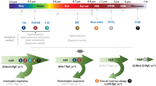
Our objective in this review is to evaluate how satellite observations have informed our understanding of terrestrial carbon balance and its key component fluxes (GPP, disturbance-induced carbon losses and net biome productivity) at both regional and global scales. We then quantified potential uncertainties of terrestrial carbon fluxes by assembling different satellite-based datasets and comparing these results with the output from an ensemble of DGVMs in TRENDY (Trends and drivers of the regional scale sources and sinks of carbon dioxide) project and the net carbon balance estimate using the latest comprehensive bottom-up carbon accounting approach (Ciais et al. 2022). We finally summarized future challenges and opportunities that could help in obtaining accurate estimates of spatio-temporal patterns of terrestrial carbon fluxes using satellite-derived observations.

2. Principles of satellite-based retrieval of terrestrial carbon fluxes

2.1. Global primary productivity

Gross primary productivity (i.e. GPP) is the total carbohydrates fixed by plants through photosynthesis. It fuels the ecosystems and is considered as the start of the terrestrial carbon cycle (Beer et al. 2010). Plant photosynthesis combines two processes known as the light-dependent reaction and light-independent reaction. During the light-dependent reaction, solar energy absorbed by the photosynthetic pigments in the green leaves is converted to biochemical energy stored in Adenosine 5’-triphosphate (ATP) and nicotinamide adenine dinucleotide phosphate (NADPH). A small fraction of energy is also reemitted as chlorophyll fluorescence during this process (Krause and Weis 1991; Porcar-Castell et al. 2014). Both ATP and NADPH generated by the light-dependent reaction are further used by the light independent reaction which converts CO₂ to carbohydrates through a series of biochemical reactions (i.e. the Calvin Cycle) (Raines 2003).

Remote sensing has long been used for GPP estimates, whose fundamental basis can be categorized into four approaches: (1) process-based models; (2) light use efficiency models; (3) machine learning based models; (4) empirical relationship with vegetation indicators. Process-based models use remote sensing retrieved ecosystem parameters (such as leaf area index, clumping index, maximum carboxylation rate at reference temperature) as input for models that represent the physiological process of photosynthesis. The most widely used process-based model is the Farquhar-van-Caemmerer-Berry (FvCB) model which considers the two major limitations of photosynthesis, i.e. RuBP regeneration and carboxylation of Rubisco, which are further mediated by the stomata responses to the environment (Farquhar, von Caemmerer, and Berry 1980). Remote sensing products are often used to describe the maximum activity of enzyme, which determines the photosynthesis of individual leaf, as well as the light distribution within the canopy, which scales the photosynthesis of individual leaf to the entire canopy. Some well-known examples include the Breathing Earth System Simulator (BESS) (Li et al. 2023; Ryu et al. 2011) and Boreal Ecosystems Productivity Simulator (BEPS) (Chen et al. 1999). These models are mechanistic, but often requires complex parameterization.

Light use efficiency models are built based on the fact that solar radiation absorbed by plants’ green leaves are the first order driving factors for photosynthesis. The energy absorbed by plants is wavelength dependent, leading to a unique signature in reflectance spectrum, from which various vegetation indices can be derived. These indices, such as NDVI or EVI, have been demonstrated to strongly related to the fraction of energy absorbed by green vegetation (Zeng et al. 2022). Together with solar radiation and a light use efficiency factor that converts solar energy to chemical energy, the product of these three factors can provide a reliable estimate of GPP (Pei et al. 2022). Some widely used datasets include MODIS GPP (MOD17) (Running et al. 2004), Vegetation Photosynthesis Model (VPM) (Xiao et al. 2004), Eddy Covariance-light use efficiency (EC-LUE) (Yuan et al. 2007).

Machine learning models have been extensively used in estimating GPP and other carbon fluxes. These models follow a data-driven concept to explore the relationship between GPP and various environmental and vegetation-related variables. Remotely sensed vegetation indices, land surface temperature and other datasets can be used as the input variables and GPP estimates at eddy covariance sites are usually considered as training targets (Jung et al. 2012). They often show quite good spatial and seasonal variation as compared to the ground observations, but the interannual variations are often underestimated.

The last kind of method is based on empirical relationship with SIF and other vegetation indicators. SIF is emitted by both photosystem II and photosystem I during the light-dependent reaction, it is strongly related to the electron transport rate and is therefore a good indicator of the energy harvest during the light-dependent reaction (Porcar-Castell et al. 2014). Considering that the reaction speed of the light-dependent reaction is often coordinated with the light-dependent reaction, SIF also has a strong relationship with the gross photosynthesis rate (Porcar-Castell et al. 2014). The global GPP can be estimated based on the empirical relationship obtained at site level. Some other indicators that are demonstrated to be strong proxies of GPP include PAR times near infrared reflectance (NIRv, a factor that better considers canopy structure effect) or kernel-NDVI (kNDVI) (Camps-Valls et al. 2021; Dechant et al. 2022). Besides the four major approaches mentioned above, some recent studies also suggest that carbonyl sulfide (OCS or COS) is a robust indicator of canopy stomatal conductance, advances in remote sensing technique can observe the atmospheric OCS concentration variations, but spatially explicit GPP estimates based on OCS is still challenging (Whelan et al. 2018).

Some of the carbon fixed by plant photosynthesis will be respired by plants (autotrophic respiration) and directly returned to the atmosphere, the rest that will be allocated to different carbon pools is known as the net primary production (NPP). Although global evidence suggests the NPP almost takes half of GPP, the ratio between these two varies with climate, soil, nutrient, plant characteristics and other environmental factors (Tang et al. 2019). Two types of models are proposed to calculate NPP. One is an empirical model similar to the LUE models, but instead of using the light use efficiency, it employed a factor that directly converts the absorbed energy to biomass increment. One example is the widely used CASA model (Potter et al. 1993). The other type of model is more physiological, which considers both maintenance respiration and growth respiration as functions of temperature. The example is the MODIS NPP (Running et al. 2004). For grassland ecosystems where plants grow annually, the aboveground NPP is often estimated as a function of vegetation indices since these indicators are strongly related to leaf area and biomass (Fang et al. 2001; Ponce-Campos et al. 2013).

When ecosystem heterotrophic respiration is also removed from the NPP, the rest is the net ecosystem productivity (NEP), which represents the carbon fixed by plants without considering the effect of disturbances. Although there is no direct way to estimate heterotrophic respiration from remote sensing, some models use simulated GPP and soil organic carbon to calculate a reference ecosystem respiration, together with environmental factors to estimate ecosystem respiration (autotrophic plus heterotrophic) (Li et al. 2023).

2.2. Anthropogenic and natural disturbances

Carbon fluxes due to ecosystem disturbance are important fluxes in terrestrial carbon balance accounting at both regional and global scales (Ciais et al. 2022; Phillips et al. 2022; Pongratz et al. 2021). Disturbances include natural ones such as lightning-ignited wildland fires (Phillips et al. 2022), wind storm (Feng et al. 2022), snow storm, insects, and anthropogenic ones such as human land use and land use change (Pongratz et al. 2021). Land use change affects carbon cycling by altering the land cover type, for example, by clearing and converting forest to cropland or grazing land, or draining wetland and converting to cropland, or the reverse processes of afforestation/reforestation or wetland restoration.

Remote sensing plays a crucial role in supporting the quantification of carbon fluxes through land use and land use change, both by mapping land use/land cover dynamics (Zhang et al. 2021) and by directly mapping changes in biomass carbon storage (Liu et al. 2015; Santoro et al. 2021). To derive carbon fluxes (carbon emission or carbon uptake) from land cover change, annual maps of land cover distribution were used as input in bookkeeping models or dynamic global vegetation models to diagnose carbon fluxes corresponding to different land cover change processes (Friedlingstein et al. 2022; Hansis, Davis, and Pongratz 2015; Song, Huang, and Townshend 2017).

The long-term monitoring of land cover change involves establishing the land cover distribution for a base year and detecting the changes from the base year to the target year (Zhang et al. 2021). The mapping of land cover distribution for a given year (or the base year) requires training samples with known land cover types and the associated spectra information, sometimes with additional supplementary information such as elevation and phenology information. A globally uniform classification model, or several regional specific models, are then trained using the training samples and input spectra features. These models are finally combined with input spectra information from satellite remote sensing to derive land cover distribution. For long-term land cover monitoring, satellite pixels with potential land cover changes are first identified (such as the Continuous Change Detection method (Zhu, Woodcock, and Olofsson 2012) and LandTrendr (Huang et al. 2009), followed by further identification of the new land cover type (Zhang et al. 2021).

The most widely used long-term series of land cover mapping by far is the ESA CCI land cover product which covered 1992–2020 (http://maps.elie.ucl.ac.be/CCI/viewer/download.php) with a 300 m spatial resolution, which was incorporated in the historical dataset of cropland and grazing land (HYDE3.2, Klein Goldewijk et al. 2017) and further used in the land use transition dataset of LUH2 (Hurtt et al. 2020) adopted by the Global Carbon Project. Another dataset of land cover with a fine classification system covering 1985–2020 with a 30 m resolution was recently released (Zhang et al. 2021). In addition, several thematic land cover map time series products were also available, including those for urban land impervious surface area (Gong et al. 2020; Liu et al. 2020) and for cropland (Potapov et al. 2022).

In terms of wildland fires, three types of information can be derived from satellite remote sensing: active fire, burned area, and fire radiative power (Mouillot et al. 2014). The active fire product provides information on temporal and spatial locations where fires are observed as active burning when satellites pass by (Giglio, Schroeder, and Justice 2016). The burned area product provides gridded information on where fires have occurred and vegetation has been disturbed (Chuvieco et al. 2018). Fire radiative power measures the radiative energy released per unit time by actively burning vegetation fires. To obtain fire carbon emissions, spatially explicit burned area data need to be combined with information about the available fuel for combustion and the combustion fraction by fire, both of which are often obtained through model simulations (Van der Werf et al. 2010). The other approach is to empirically convert the observed fire radiative energy, calculated by integrating the fire radiative power over time, directly to biomass consumption by fire (Kaiser et al. 2012).

The detection of active fire mainly uses the reflectance in the mid-infrared (MIR) bands (3–5 μm). The most widely used MODIS active fire product used the reflectance for the wave length of 4 μm and the Stefan-Boltzmann law to invert the surface temperature of the observed satellite pixel, followed by applying spatially varying thresholds to detect active fire (Giglio, Schroeder, and Justice 2016). The fire radiative power algorithm is based on the same principle and translates the difference in the reflectance of MIR between the active fire pixel and the background unburned pixels to the energy release using empirical relationships (Wooster et al. 2005). The burned area algorithm examines temporal changes in a burn-sensitive vegetation index and then compares such changes with those of active fire pixels and the unburned background pixels to identify the probability of a given satellite pixel being burned (Giglio et al. 2018). The burn-sensitive index uses the contrast between the near infrared (NIR) and the short-wave infrared (SWIR) bands, where vegetation has a high and low reflectance, respectively (Giglio et al. 2018).

2.3. Satellite-based inversion of net biome production

The temporal and spatial variations of atmospheric CO₂ abundance are influenced by the dynamics of net CO₂ exchanges between the Earth’s surface and the atmosphere, convolved with atmospheric transport. Thus, dense CO₂ measurements can be used to deduce the timing, location, and intensity of CO₂ fluxes. The efforts of using remote sensing techniques to retrieve atmospheric CO₂ concentrations started in the 1980s, equipping sensors onboard satellites to measure spectra of reflected sunlight or emitting thermal radiation by the Earth within the CO₂ absorption bands. The current operational satellites dedicated to CO₂ monitoring all use high-resolution spectrometers at short wavelength infrared (SWIR) bands, due to their relatively higher sensitivity to CO₂ variations in the lower troposphere than thermal infrared (TIR) sensors. The spectra recorded by satellite-borne sensors are analyzed by a retrieval algorithm, fitting the spectral lines within absorption bands, to quantify the clear-sky column-average CO₂ dry air-mole fractions (XCO₂), which also account for atmospheric and surface conditions, as well as the optics and electronics properties of the sensors (O’dell et al. 2018). These XCO₂ data are assimilated in atmospheric inversion systems, which use atmospheric transport models to link the CO₂ fluxes and XCO₂ and solve for the optimal spatial and temporal variations of CO₂ fluxes that match the spatial gradients and temporal changes of CO₂ abundance, accounting for the large-scale horizontal transport and vertical mixing of the atmosphere (Chevallier et al. 2019; Jin et al. 2023). XCO₂ signals are impacted by both natural and fossil fuel CO₂ fluxes. In most atmospheric inversions, the model input of fossil fuel CO₂ emissions is assumed to be perfectly known without any uncertainty, and only the fluxes from natural ecosystems are inversely solved. The inversion problem is generally ill-conditioned as current satellite observations are not dense enough to cover ubiquitous CO₂ fluxes, and atmospheric inversions is usually performed based on Bayesian inference, using some prior knowledge to provide additional information on flux estimates (Rayner, Michalak, and Chevallier 2016).

3. Current status of satellite-derived terrestrial carbon fluxes

3.1. The GPP pattern and its trend

By making use of various remote sensing datasets, we provided a satellite-derived estimate of an average global GPP of 134 PgC yr⁻¹, with a standard deviation of 14 PgC yr⁻¹ among different datasets during the period 2001–2022 (Figure 2). This satellite-derived estimate is consistent with the multi-model ensemble mean of GPP from TRENDY S3 simulations which include the impacts of climate change, rising atmospheric CO₂ and land use changes (131 ± 10 PgC yr⁻¹) (Figure 3).

Figure 2. Spatial patterns of mean and standard deviation of annual gross primary production (GPP) and its trends in the last two decades. (a and b) the mean and standard deviation annual GPP from different GPP products, (c and d) the mean and standard deviation of trends in annual GPP in the last two decades from different products, and (e) the time series of global annual GPP for the four different GPP products (MODIS, BESS, GOSIF and PML), the flux-derived GPP, and multi-model mean from TRENDY project. Here the flux-derived GPP data (https://doi.org/10.3334/ORNLDAAC/1835) is the upscaling of eddy covariance flux measurements from selected FLUXNET 2015 to the global scale in a machine learning algorithm using nadir bidirectional reflectance distribution function (BRDF)-adjusted reflectances (NBAR) product as inputs.

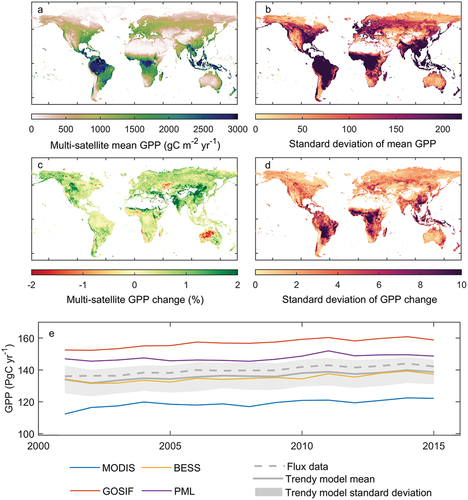
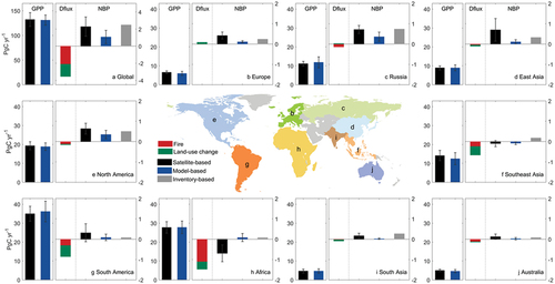
Figure 3. The comparison of terrestrial carbon fluxes among satellite derivation, model simulations and inventory-based approach at both regional and global scales. GPP and NBP are gross primary productivity and net biome productivity, respectively, and Dflux represents carbon fluxes associated with wildfire disturbance and land-use change. The GPP and NBP in black represents the satellite-based estimates during periods 2000–2022 and 2015–2020, respectively. The NBP in gray stems from the latest comprehensive bottom-up carbon accounting approach and this value is calculated as the sum of inventory-based carbon stock changes and lateral carbon fluxes (crop and wood trade, and riverine-carbon export to the ocean) during the period 2000–2009. The model-based GPP and NBP during the period 2010–2018 are derived from TRENDY model simulations under S3 simulation scenario (with time-varying climate, CO₂ concentration and land-use).

Although satellite-derived GPP datasets have a similar spatial pattern in terms of annual mean, differences exist, especially for the tropical regions (e.g. South America and Africa), where annual GPP are the highest across the globe. By separating the global land into different regions, South America and Africa, where mainly distributes tropical forests and savannahs, altogether account for nearly half of the global terrestrial GPP. Meanwhile, the SIF-based GPP (GOSIF: Global OCO-2 SIF based GPP) estimates over both South America and Africa are more than 30% and 10% larger than results from the MODIS estimate (using traditional remotely sensed vegetation indices) and state-of-the-art carbon cycle models, respectively (Figure 2). In addition, croplands in the midwestern United States generally have the highest peak photosynthesis because of the role of management. While, crop GPP is underestimated in products which uses NDVI or fPAR as an input, and is more reasonably approximated based on EVI, NIRv, and SIF that could well capture the effect of canopy structural complexity on GPP. This result is anticipated since vegetation indices especially NDVI could be saturated over tropical forests and highly productive crops, and would then have nonlinear relationships with GPP (Badgley et al. 2017; Camps-Valls et al. 2021). By contrast, the saturation problem of SIF and NIRv (the proportion of reflected near-infrared radiation attributable to vegetation) in the tropical region has been significantly eliminated.

In the last two decades, there is a general increasing trend in global GPP, with a mean value of 0.45 ± 0.11 PgC yr⁻², based on the four satellite-based products during the period 2001 to 2015. This satellite-derived estimate is generally consistent with the multi-model ensemble mean from TRENDY models (0.49 ± 0.10 PgC yr⁻²) during the period 2001 to 2015 (Figure 2). However, the magnitude of the trend in global GPP varies across different satellite products, with the estimate of GPP from Penman – Monteith – Leuning model (PML, He et al. 2022) being the smallest (0.31 Pg C yr⁻²) while the other three estimates ranging between 0.43 and 0.58 Pg C yr⁻². In terms of spatial pattern, there is an almost ubiquitous increase in GPP, except the Australia and Central Asia in the past two decades, with a larger increase especially in south Asia, east Asia and other tropical regions and a relatively smaller one in the Northern Hemisphere. Meanwhile, the inter-product discrepancy in GPP trends becomes larger in South America and Africa, with MODIS-based trends being almost twice as large as those from GOSIF and BESS (Breathing Earth System Simulator-based GPP) (Figure 2). Such divergence in GPP trend reflects how the fertilization effect of rising CO₂ and the impact of environmental stress (e.g. atmospheric vapor pressure deficit) on plant physiology was considered in the satellite-derived product.

3.2. Carbon fluxes due to anthropogenic and natural disturbances

Land-use change and increasing natural disturbances such as wildland fires and insects are important processes that generally reduce net biome uptake. First, human land use and management represent important anthropogenic disturbances to terrestrial ecosystems. Deforestation followed by conversion to croplands, converting grassland to cropland, peatland draining and burning, and forest harvest, on one hand, release carbon stored in biomass and soil into the atmosphere (Houghton 2012; Poeplau et al. 2011). On the other hand, active afforestation, cropland abandonment and forest regrowth following harvest contributes to carbon sink (Chazdon et al. 2016; Deng et al. 2014).

Historically, since 1850 both tropical and non-tropical regions have been losing forest being converted to agricultural land until about 1950s, when forest loss was reversed in non-tropical regions (mainly northern hemisphere) whereas forest loss kept accelerating in non-tropical regions (Houghton and Nassikas 2017). For 2001–2020, forest loss was mainly found in Africa, Southeast Asia and Latin America (including Democratic Republic of the Congo, Indonesia, and Brazil), whereas forest recovery was found in northern extra-tropics including Europe, USA and China (Grassi et al. 2023).

Globally, the net effect of historical land use and land use change was a carbon source of 1.2 ± 0.7 Pg C yr⁻¹ for the most recent decade of 2012–2021 (Friedlingstein et al. 2022). The cumulative emissions from land use change for 1850–2022 reached 206 ± 60 PgC, accounting for 30% of the total anthropogenic emissions (Friedlingstein et al. 2022). About 80% of the cumulative emissions come from agricultural expansion at a cost of forest and natural grasslands, with the remaining mainly coming from industrial and fuel wood extraction. Regionally, emissions mainly come from tropical Africa, Latin America and South and Southeast Asia, whereas carbon uptakes by land use change are found in North America, Europe, former Soviet Union countries, and China (Houghton and Nassikas, 2017).

Second, wildland fire is a widespread disturbance form spanning across different ecosystems on Earth including forests, grasslands, and croplands (Giglio et al. 2018). Remote sensing-based burned area provides the fundamental data needed for a bottom-up quantification of global and regional fire carbon emissions (Chuvieco et al. 2016; van der Werf et al. 2017; Ramo et al. 2021). The mainstream burned area datasets for global application have medium spatial resolution ranging from 250 m to 500 m (Giglio et al. 2018; Lizundia-Loiola et al. 2020). The global total burned area according to the state-of-the-art medium-resolution products range between 345 Mha yr⁻¹ (1Mha = 10⁶ ha) and 468 Mha yr⁻¹ for 2002–2012 (Hantson et al. 2020). Ninety percent of the burned areas are found in the tropics of 30ºS–30ºN being dominated by savanna vegetation (76% of the global total), with the remaining mainly being found in Eurasian grassland and cropland, and temperate and boreal forests. Of the savanna fires, 84% are contributed by African savanna, 11% by Australian savanna and 5% by American savanna. Cropland fires account for about 10% of the total global burned area.

Global wildland fires emit on average 2.2 ± 0.3 Pg C per year (with the uncertainty calculated as the standard deviation over time) into the atmosphere during 1997–2016 according to the most widely used GFED4s dataset (van der Werf et al., 2017). Similar to the dominance by the tropics in burned area, 84% of global fire carbon emissions have an origin in the tropical region between 23.5ºN and 23.5ºS, and 62% come from tropical savannas (van der Werf et al., 2017). Fire emissions associated with tropical deforestation reached about 0.3 PgC yr⁻¹, with additional emissions of 0.07 PgC yr⁻¹ from peatland burning in Southeast Asia. Temperate and boreal forests collectively contribute about 10% of the global fire carbon emissions, and cropland fires contribute about 6%.

3.3. Global and regional net biome production

The use of a top-down atmospheric inversion method combined with satellite-derived column-integrated CO₂ retrievals could reveal new information about carbon cycle in a global coverage. Here, we used inverted net carbon exchange from OCO-2 Multi-model Intercomparison Project (https://gml.noaa.gov/ccgg/OCO2_v10mip/index.php), wherein 14 models conducted experiments assimilating OCO-2 column-averaged dry-air mole fraction (XCO₂) retrievals (2015–2020) (Byrne et al. 2023; Yang et al. 2023). The magnitude and uncertainties of inversion-based estimates of net biome productivity during 2015–2020 were shown at both global and regional scales (Figure 3). At the global scale, terrestrial ecosystems are a strong sink of 2.28 ± 1.12 PgC yr⁻¹ during the period 2015–2020.

The contributions of each region to global NBP differ in magnitude. The extra-tropics in both hemispheres are carbon sinks (3.02 ± 0.88 Pg C yr⁻¹), while the tropics is a carbon source (0.89 ± 0.44 Pg C yr⁻¹). Due to the mixing of atmosphere and the nature of XCO₂ that integrates air coming from various regions throughout the atmospheric column, the consistency among different inversion models decreases with the spatial scales (Crowell et al. 2019; Peiro et al. 2022). In particular, there are considerable uncertainties in estimate of CO₂ fluxes over Southern Tropical South America (0.04 ± 0.24 PgC yr⁻¹), Southern Tropical Africa (−0.10 ± 0.16 PgC yr⁻¹) and Eurasia Temperate (−0.47 ± 0.63 PgC yr⁻¹) (Figure 3). Estimates of country-level flux generally agree among models for well-sampled large extratropical countries (e.g. USA, −0.45 ± 0.16 Pg C yr⁻¹; Russia, −0.68 ± 0.18 Pg C yr⁻¹), but not for mid-sized countries (e.g. Australia, −0.11 ± 0.12 Pg C yr⁻¹; Spain, −0.03 ± 0.02 Pg C yr⁻¹) and frequently cloudy countries (e.g. China: −0.58 ± 0.45 PgC yr⁻¹; India: −0.17 ± 0.11 PgC yr⁻¹) (Schuh et al. 2022; Wang et al. 2022).

We further compared satellite-based inverted estimates (2015–2020) to the latest comprehensive inventory-based estimate (2000–2009) and process-based model simulations (2010–2018) by splitting the globe into ten different regions (Figure 3). Note that the use of different periods complicated the NBP comparison, while its impact on the result was expected to be small. To be properly compared with the inverted estimate of NBP, we used inventory estimates of carbon stock change by including lateral carbon fluxes from crop and wood trade and riverine-carbon export to the ocean during the period 2000–2009 (Ciais et al. 2022). The global inverted NBP is generally consistent with inventory-based approach, but is twice as large as that from TRENDY models under S3 simulation scenario with timing-varying climate, CO₂ and land use. The discrepancy between atmospheric inversion and model simulations would partly arise from the poor process representation of carbon fluxes associated with disturbance especially land-use changes in models. This also explained why the net terrestrial carbon balance updated annually by Global Carbon Project was calculated as the sum of NBP from TRENDY models using S2 simulations (with time-varying climate and CO₂ but constant land use) and land use-induced net CO₂ emissions from bookkeeping models. The satellite-based atmospheric inversion agreed with inventory-based approach that the largest carbon sink occurred in North America and Russia, but disagreed that Africa was a large carbon source (Figure 3).

In addition, the satellite-based inversions by assimilating XCO₂ retrievals hold the potential to reveal the impact of extreme events on land carbon fluxes anomalies. During 2015–2016 El Niño events, the global carbon sink was reduced by ~ 1 PgC year⁻¹ based on satellite-based inversions by assimilating GOSAT and OCO-2 XCO₂ measurements (Crowell et al. 2019; Palmer and Ruhi 2019). At the regional scale, the satellite-based inversions detected a reduction of carbon sink in Europe in 2012 (ranges between −112 and 170 TgC yr⁻¹) and 2015 (ranges between −92 and 218 TgC yr⁻¹) due to drought conditions. In contrast, inversions assimilating observations from the European network of surface stations did not capture the carbon sink reduction in 2015 (W. He et al. 2023)highlighting the usefulness of remote sensing in monitoring the dynamics of CO₂ fluxes.

3.4. A summary of terrestrial carbon balance

By synthesizing satellite-based estimates of GPP, NPP (MODIS), disturbance-associated carbon fluxes and NBP, we have listed all component fluxes of terrestrial carbon balance at both regional and global scales (Table 1). First, by summing up disturbance-associated carbon fluxes, lateral carbon fluxes (crop and wood trade, and riverine-carbon export to the ocean) (Ciais et al. 2022) and NBP, the global net ecosystem productivity (NEP) due to climate change, rising CO₂ and other factors such as nitrogen deposition amounts to the sink of CO₂ of ~ 6.81 PgC year⁻¹.

Table 1. The main flux components of global and regional carbon balance. Note that only GPP, NPP, disturbance flux and NBP are remotely sensed. Other components such as soil and ecosystem respiration, and NEP are deduced from remotely sensed fluxes. Negative sign indicates a carbon source. The time periods used to obtain GPP, disturbance flux and NBP are 2000–2022, 2012–2021 and 2015–2020, respectively.

Region	Main flux component (PgC yr^−1)									Area (million km^2)
	GPP	MODIS NPP	Disturbance	NBP	NEP	Soil respiration	Ecosystem respiration	Disturbance/NEP (%)	NEP/GPP (%)
Europe	6.7 ± 0.7	3.9	0.08	0.42 ± 0.17	0.27	−3.6	−6.4	30.2	4.0	5.19
Russia	11.2 ± 1.3	6.1	−0.12	0.72 ± 0.2	1.01	−5.1	−10.2	−12.0	9.1	17.02
East Asia	8.9 ± 1.1	4.6	−0.11	0.7 ± 0.55	0.84	−3.8	−8.1	−13.3	9.4	11.61
South Asia	4.7 ± 1.0	1.7	−0.09	0.17 ± 0.12	0.41	−1.3	−4.3	−22.7	8.7	4.49
Southeast Asia	14.9 ± 2.7	6.0	−0.66	−0.1 ± 0.15	0.76	−5.2	−14.1	−87.8	5.1	4.5
Africa	27.8 ± 3.0	12.5	−1.48	−0.69 ± 0.41	0.86	−11.6	−26.9	−172.1	3.1	29.63
North America	19.7 ± 2.1	10.2	−0.16	0.64 ± 0.27	0.95	−9.2	−18.7	−16.8	4.8	22
South America	35.2 ± 3.9	15.9	−0.86	0.32 ± 0.44	1.44	−14.5	−33.8	−59.3	4.1	17.9
Australia	5.0 ± 0.6	3.0	−0.14	0.12 ± 0.13	0.28	−2.7	−4.7	−51.4	5.5	7.7
Globe	134.1 ± 14.0	63.9	−3.55	2.28 ± 1.12	6.81	−57.1	−127.3	−52.1	5.1	120.04

Second, since there were no direct satellite observations of respiration fluxes, ecosystem respiration was calculated as a residual between satellite-derived GPP, NBP, disturbance-associated fluxes (Figure 3) and lateral carbon fluxes (Ciais et al. 2022). The NPP from MODIS data, which is combined with inferred ecosystem respiration, was further adopted to estimate soil microbial respiration at both regional and global scales. The inferred ecosystem respiration (127.3 PgC yr⁻¹) is higher than that from data-driven empirical models using global eddy covariance flux measurements (95 to 114 PgC yr⁻¹) (Yu et al. 2022) but consistent with process-based model simulations (136 ± 37 PgC yr⁻¹) (Li et al. 2018). In addition, the inferred global soil microbial respiration (57.1 PgC yr⁻¹) was also higher than that (33–46 PgC yr⁻¹) estimated using the inventory-based approach (Ciais et al. 2022).

Third, according to calculated carbon flux components, we could infer that global ecosystem carbon use efficiency (CUEe; ratio of NEP to GPP) is ~ 5.1%, with relatively high ones in the Northern Hemisphere especially East Asia (~9.4%) and Russia (~9.1%), but relatively low ones in tropical region such as Africa (~3.1%) and South America (~4.1%) (Table 1). The highest CUEe in East Asia could be associated with intensive reforestation and afforestation practices in southern China (Forest management in southern China generates short term extensive carbon sequestration), leading to greater carbon sequestration capacities. The lower CUEe in hot tropical regions would suggest enhanced respiration losses due to a warming-induced acceleration of decomposition, resulting in less efficient carbon storage in ecosystems. Furthermore, disturbance-induced carbon emissions have offset ~ 60%, ~88% and ~ 172% of net ecosystem productivity due to climate change and rising CO₂ concentration in South America, Southeast Asia, and Africa (Table 1), respectively, highlighting the importance role of disturbance in regulating tropical carbon balance.

4. Key questions

Our synthesis of satellite-derived estimates of main carbon flux components are subjected to great uncertainties. Although the estimate of GPP is converging at the global scale among different data sources (Figures 2 and 3), there is relatively low confidence in the estimate of regional GPP and its long-term trend, especially in tropical forests and semi-arid regions. This is mainly due to missing or under-parameterized processes, such as climate-induced physiological adjustments and CO₂ fertilization effect, in the current satellite-based framework to retrieve GPP.

In comparison to the latest comprehensive bottom-up carbon budget accounting at both regional and global scales (Ciais et al. 2022), the satellite-based inversion is relatively robust in the estimate of carbon budget, especially at the global scale. While the satellite-based inversions still have a relatively large inter-model spread and its multi-model ensemble mean also largely deviated from the previous inventory-based estimate in some regions such as Africa and Southeast Asia (Figure 3), highlighting the necessity to reduce manifold sources of uncertainties such as in inversion schemes and atmospheric transport models (Baker et al. 2006; Gurney et al. 2016).

Furthermore, we realized that NBP simulations from process-based models have a large deviation from satellite derivations and the bottom-up approach at both regional and global scale (Figure 3). One source of model uncertainties arises from poor parameterizations of the partitioning of the photosynthetic products into different functional carbon pools, and carbon residence time in both biomass and soils (Friend et al. 2014; He et al. 2016). Another major source of these model uncertainties would arise from underrepresentation of processes or mechanisms which determine ecosystem responses and recovery after natural (e.g. fires, climatic extremes) and human disturbances (e.g. land-use change, land management). Although an integration of satellite observations with emission and removal factors can help determining carbon fluxes associated with the main disturbance types such as wildfires and land-use change (Figure 3), these numbers are prone to large uncertainties due to an incomplete satellite mapping of different types of disturbances (e.g. abiotic factors such as insect outbreak) or a poor understanding of processes such as the burning of soil carbon pools in the calculation of gross carbon emissions. It is then a highly necessity to improve satellite-based estimates of disturbance-associated carbon fluxes and their drivers, and improve them in the next generation of process-based models. There are also inaccuracies in atmospheric transport models that could lead to notorious uncertainties in top-down estimates of regional carbon sources and sinks (Schuh et al. 2019). These deficiencies were also responsible for an inconsistent estimate of main terrestrial carbon fluxes between satellite-based inversion and process-based model simulations. In addition to resolving these model discrepancies, we also needed to address the large inconsistencies of terrestrial carbon fluxes such as primary productivity and respiration among different sources of observation-based datasets (Jian et al. 2022), since these datasets are crucial to the development and parameterization of specific model processes. Based on our data synthesis, we have identified several knowledge gaps that require further research in the field of remotely sensed terrestrial carbon fluxes.

Q1:

How to incorporate physiological effects to improve confidence in detection of long-term change in GPP?

Terrestrial photosynthesis is increasing with elevated atmospheric CO₂ concentrations (Fatichi et al. 2016; Zhu et al. 2016) but decreased with physiological stress such as drought and heat (Qiao and Xia 2024; Stocker et al. 2019). Traditional reflectance-based photosynthesis products typically combined satellite-derived canopy changes (such as leaf area index and Normalized difference vegetation index) with empirical parameterizations of the effects of climatic stress and increasing CO₂ concentrations on photosynthesis to estimate GPP.

While, climatic stress such as drought and heat could provoke changes in plant physiology without affecting canopy structure (Stocker et al. 2018). Such physiological climatic stress-induced reduction in GPP was then not be captured by traditional reflectance-based GPP products. SIF, which is a direct measure of light re-emitted from chlorophyll during the light reactions of photosynthesis, is not only driven by chlorophyll absorbed PAR, but also contains information on subsequent energy partitioning which is directly regulated by plant physiological stress (Kimm et al. 2021). SIF then integrates both structural and physiological processes of a vegetation canopy, and provides an instantaneous measure of individual or compound influence of climatic stress on photosynthesis. Looking forward, OCO-3 onboard the International Space Station (ISS) provided diurnal SIF observations, a timescale when physiological stress decouples from structure and biochemical changes. These diurnal SIF observations could help separate individual components of climatic stress on structural and physiological processes, which could be coupled at the relatively coarse temporal resolution such as month (Magney, Barnes, and Yang 2020).

Although the use of SIF would be effective in representing climatic stress on photosynthesis, only relying on the combination of SIF and reflectance-based indices (LAI and/or fAPAR) to track GPP could not fully account for the CO₂ fertilization effect on photosynthesis. Increases in atmospheric CO₂ concentration could stimulate photosynthetic uptake via the two direct physiological pathways: enhancing light use efficiency (LUE, changes in photosynthesis per unit light absorbed) and water use efficiency (WUE, changes in photosynthesis per unit water loss through transpiration), and one direct pathway: increasing LAI and then fAPAR. The combined use of reflectance-based canopy changes (LAI or fAPAR) with SIF, which can be utilized to constrain LUE, and thermal infrared-derived land surface temperature, which can estimate transpiration and provide a constraint on WUE, has the potential to fully capture photosynthesis due to the rising CO₂ (Smith et al. 2019).

Q2:

Could satellite data tell us whether climate change induced an enhanced tree mortality?

Accumulating evidence suggested that climatic extremes such as drought and heatwaves could lead to tree mortality that is defined as “the point of no return” for functioning for the whole-plant, including the loss of living tissues and failure of the hydraulic structure to conduct water (Anderegg et al. 2015; Hartmann et al. 2018). All this knowledge is mostly derived from a compilation of reported idiosyncratic tree mortality cases (Allen et al. 2010; Allen, Breshears, and Mcdowell 2015; Hartmann et al. 2018). These ground-truth data stimulated our recognition of internal physiological pathways such as hydrologic failure and carbon starvation in triggering tree mortality (Hartmann et al. 2018), but are very limited in offering a spatially explicit characterization of spatiotemporal trends in tree mortality rates, because of their geographical observational bias and non-regular update. Although a few hundred ground-based plots were recently upscaled to continental-scale domain using climatic drivers (Yu et al. 2022), these extrapolations must be evaluated with due rigor until studies can demonstrate that these mortality events are climate-driven and adequately sampled across the domain (Chambers et al. 2009).

How tree mortality rates are linked to climate change vary across ecosystems and across the globe and therefore remains elusive. As climate warms, compared to trees in high latitudes, trees in low latitudes such as tropics live very close to their thermal optima (Huang et al. 2019), and would potentially face greater mortality risks in a hotter future with an occurrence of drought due to more frequent El Niño events. On the other hand, tropical forests have more diverse in species composition than other forests, and could then enhance forest resistance to climatic extremes via complementarity effect among species (Liu et al. 2022). Without long-term monitoring, we could not quantify deviations from normal background mortality rates and determine the extent to which climate change has affected the size and number of tree mortality events. In addition to quantifying the cross-biome pattern of mortality excess to climate change, how vegetation recovered in the mortality gap remains unquantified. Bridging this knowledge gap will help accurately estimating the role of tree mortality in the evolution of regional carbon balance, particularly in temperate and tropical regions.

To resolve these scientific concerns, a frequently updated global tree mortality event map is a highly necessity. The remote sensing with time series of imagery provides a promising avenue, due to their capacities to provide repeated observations over large areas at a higher temporal resolution and lower cost than terrestrial surveys. However, traditional satellite data, often at a low data resolution, are still insufficient for detecting small-scale tree mortality (e.g. less than 0.1 ha) with its occurrence orders of magnitude higher than that of larger-scale mortality (Espírito-Santo et al. 2014). Although the multi-temporal data from very high-resolution satellites such as the 0.7-m resolution QuickBird have been used to measure tree death rates in the tropical rainforests (Clark et al. 2004), they are often fraught with sun-geometry errors. The emerging satellite techniques such as repeated small-footprint airborne lidar acquisitions were recently demonstrated to hold a great promise to track the demography of millions of trees over a vast area (Dalagnol et al. 2021; Huertas et al. 2022). Such multi-temporal Light Detection and Ranging (LiDAR) onboard upcoming satellites has the potential to detect structural or compositional changes of forests and well separate the signal of overstory tree mortality from understory greening in response to canopy opening.

Q3:

How to develop a satellite-based framework to constrain belowground carbon dynamics?

While temperature is a strong driver of respiration, previous studies generally developed a statistical model of in situ measured respiration rates to land surface temperature, soil moisture and vegetation growth as a proxy of soil carbon inputs across sites and years, and then combined this statistical-based approach with different sources of satellite observations to provide a temporally consistent and spatially explicit map of ecosystem respiration (Tang et al. 2020). But such empirical-deduced respiration rates from satellite observations was questioned because the land surface temperature is not an exact measure of soil temperature but the radiative skin temperature of the land derived from infrared radiation (J. Xiao et al. 2019).

The retrieval of nighttime XCO₂ from emerging satellites, such as the Atmospheric Environmental Monitoring Satellite (AEMS) carrying an Aerosol and Carbon Detection Lidar (ACDL) instrument launched by China in April 2022, would potentially provide a direct observational constraint on the nighttime CO₂ fluxes or respiration. We could derive daytime respiration from nighttime respiration by assuming that the responses of respiration to temperature and other biotic and abiotic drivers behaves similarly during day and night. Specifically, we estimated daytime respiration using machine learning algorithms that link satellite-constrained nighttime respiration with temperature and other biotic and abiotic drivers, as attempted by eddy covariance CO₂ flux partitioning algorithms that disentangle net CO₂ fluxes into component fluxes of photosynthesis and respiration (Reichstein et al. 2005).

Q4:

How to clearly separate biospheric CO₂ fluxes from anthropogenic CO₂ emissions in satellite-based atmospheric inversions?

The atmospheric inversions generally assumed that fossil fuel CO₂ emissions have zero uncertainty. But estimates of fossil fuel CO₂ emissions at both city and national scales would be subjected to systematic biases due to different input inventory data, inconsistency of CO₂ emission factors for fuels used in greenhouse gas inventories (Liu et al. 2015), and the use of distinct system boundaries in describing emissions (including or not cement manufacturing and nonenergy products) (Ciais et al. 2010), especially for developing countries (Andres, Boden, and Higdon 2014). These biases would then propagate into the estimate of terrestrial CO₂ fluxes in satellite-driven CO₂ atmospheric inversions (e.g. Saeki and Patra 2017), since the spatiotemporal gradient of XCO₂ contains signals of CO₂ fluxes from both natural and anthropogenic origins.

Currently, the inventories of fossil fuel CO₂ emissions are largely under-constrained by independent observations, and these uncertainties would then restrict our precise understanding of natural carbon cycle through atmospheric inversion. While the OCO-2 and OCO-3 satellites showed the potential value to estimate fossil fuel emissions from individual large fossil fuel power plants or cities occasionally (Nassar et al. 2017, 2021; Reuter et al. 2019), these existing missions were not specifically for anthropogenic CO₂ emissions monitoring, and the number of revisits were still not enough to constrain worldwide anthropogenic CO₂ emissions within a desired uncertainty. Some planned missions are going to explore new observing strategies to improve the coverage and resolution of XCO₂ observations, in order to separate XCO₂ signals from natural fluxes and fossil fuel emissions. These new-term efforts include the MicroCarb mission led by the French Space agency/Centre National d’Études Spatiales, a constellation of three satellites of the Copernicus Anthropogenic Carbon Dioxide Monitoring (CO2M) mission led by the ESA and the European Commission and the GOSAT-GW mission led by the National Institute for Environmental Studies, as well as the AEMS-2 and TanSat-2 missions being discussed by China.

In addition, accurate measurements of naturally occurring radioisotope (¹⁴C) from air samples, which reflects the contribution from carbon in fossil fuels and cement manufacturing completely devoid of ¹⁴C, could help disentangling fossil fuel combustion from natural sources and sinks by combining them with atmospheric transport models. The measurements of atmospheric¹⁴C have been considered as an independent and objective approach to evaluate emission inventories. The radiocarbon measurements in surface CO₂ observations have been widely adopted by the United States to reduce uncertainties on regional fossil-fuel CO₂ emissions at national (Basu et al. 2020) and city scales (Miller et al. 2020). In addition, the Integrated Carbon Observation System (ICOS) of Europe is also setting up a dense network of dozens of surface stations measuring ¹⁴C in atmospheric CO₂. The complementary constraints on fossil fuel CO₂ emissions from both surface and satellite observations will improve the application of atmospheric inversions in accurately estimate natural CO₂ fluxes.

Q5:

How to advance satellite-based mapping of ecosystem disturbances to better quantify their impacts on carbon balance?

Great uncertainties remained in global and regional land use changes over the past decades and the uncertainty was even larger when coming back further into the past. A key source of confusion is that different products use different classification systems, making it difficult to compare them and use these products in vegetation models. Previous studies show that land management can have similar impacts on surface temperature than land use change (Luyssaert et al. 2014), but land management information is still lacking in most remote sensing products. For example, to date, there is no publicly available product on the distribution of different cropland types and their associated management. Hence, one of the key future improvements in land cover mapping is to develop long-term land cover products with management information and with a harmonized classification system.

In addition, current medium-resolution burned area datasets with a global coverage are known to very likely underestimate burned area (Boschetti et al. 2019, RSE). For example, a recent analysis used Sentinel-2 images to show that MODIS-based 500 m data can underestimate burned area in Sub-Saharan by up to 80% (Ramo et al. 2021, PNAS). Increasing the spatial resolution of burned area products thus represents an important direction in the future to improve estimating both burned area and fire carbon emissions. On the other hand, the need for burned area data of long-term temporal coverage has long been stressed by the carbon cycle modeling community (Mouillot et al. 2014). The gridded burned area data with a global coverage now can date back as early as 1982 but with a coarse resolution of 0.05º (Otón et al. 2021).

Besides wildfires and land-use changes, abiotic agents (including insects), wind storms, snow storms are examples of other forms of disturbances that influence the forest carbon cycle. Future climate change is expected to increase the frequency and extent of these disturbances and the interactions among them (Anderegg et al. 2020). However, mapping the spatial and temporal distribution of these disturbances using remote sensing at a regional scale is still rudimentary, and has not yet been realized at a global scale. Although forest cover loss and forest disturbance mapping have been available for global (Hansen et al. 2013) and regional scales such as the USA (Zhao et al. 2018) and Canada (White et al. 2017), attributing forest disturbance into different agents lagged behind. In particular, identifying sporadic and partial forest loss due to drought, wind and insect disturbances is challenging, with only case studies for specific regions being reported (Senf et al. 2020). Hence, remote sensing capacity needs to be expanded in the future to provide temporally-consistent and spatially-explicit mapping for all key forest disturbances to allow monitoring of their carbon effects.

Q6:

How do we monitor directly more accurately carbon emissions from fires?

Current estimates of fire-induced carbon emissions are often carbon losses resulting from the burning of aboveground biomass or litter (Randerson et al. 2012). However, fires could also penetrate into the carbon-rich soil organic layers, leading to considerable carbon emissions, especially in tropical and boreal peatlands (Page et al. 2002; Walker et al. 2020). As peatland fires predominantly burn underground, their detection through satellites is challenging, and is complicated by the presence of thick smoke plumes that further hampers effective monitoring. Although the IPCC guidelines offer combustion coefficients to estimate CO₂ emissions from peatland fires (Hiraishi et al. 2014), these parameters would have been affected by environmental conditions such as soil moisture conditions and then have a large spatio-temporal variation (Heil and Silva Bueno 2007; Rodriguez Vasquez et al. 2021). Consequently, despite employing satellite-based burned area products and experienced equations, accurately estimating carbon emissions from peatland fires remains challenging to date.

An alternative and potent approach to quantify fire-induced carbon emissions involves utilizing satellite observations of atmospheric carbon monoxide (CO) (Liu et al. 2013). For example, data from the Measurements of Pollution in the Troposphere instrument (MOPITT) (Deeter et al. 2019) can be leveraged for this purpose. CO that is emitted alongside CO₂ during fires, could serve as a crucial tracer for fire combustion. By employing CO₂-to-CO combustion ratios, it becomes feasible to use satellite-based fire CO emissions to infer fire-induced CO₂ emissions (Zheng et al. 2021). This method offers the opportunity to estimate CO₂ emissions resulting from both vegetation biomass burning and the burning of soil organic layers.

Q7:

How satellite observations could be used to develop a satellite-informed model for near-term prediction and long-term projection of carbon balance?

Although we are now in a golden age of observing global carbon cycle from various satellite instruments, near-term prediction (nowcasting and forecasting) and long-term projection of terrestrial carbon balance still relied on process-based models, which show disagreements due to great uncertainties in model structure and process description. Combining satellite imagery with machine learning could be used in prediction tasks, but this black-box nature of data-driven predictions generally lacks physical constraints (such as energy and water conservations), and could not offer reasonable extrapolation outside the range of training conditions (Reichstein et al. 2019). Developing a satellite-informed physical-based model to improve projections of carbon cycle evolution is therefore necessary.

In the classical model-data integration framework, satellite observations were commonly used to either constrain the model’s initial state or optimize parameters associated with carbon cycling processes. In terms of constraining the model’s initial state, the flow of carbon among pools is strongly affected by state variables, and nudging modeled state variables such as carbon stock toward satellite observations at a certain point in time and space in process-based models would increase the simulation accuracy of evolution in carbon fluxes. Such a nudging technique needed a more accurate and robust estimate of ecosystem state variables such as aboveground biomass and soil carbon stock. But current optically-based estimates have a tendency to underestimate biomass stock in dense humid forest but overestimate it in sparsely-vegetated ones (Braghiere et al. 2020). The space-borne LiDAR, a laser-based remote sensing technology, provides three-dimensional data on vegetation structure e.g. vegetation height, canopy density, and vertical distribution, which enables precise estimation of biomass (Reichstein et al. 2019). In contrast, the satellite-based estimate of soil carbon stock is still in fancy, and studies are emerging to estimate surface soil carbon stock in tundra using backscatter values from synthetic aperture radar in C-band that relates to soil properties especially under frozen conditions (Bartsch et al. 2016).

In terms of optimization of model parameters, the common approach is to use satellite-derived estimates of vegetation properties such as leaf area index, the fraction of absorbed photosynthetically active radiation, and sun-induced fluorescence (Bacour et al. 2015; Forkel et al. 2019; MacBean et al. 2015; Migliavacca et al. 2009) to constrain parameters associated with photosynthesis, phenology, carbon turnover rate and carbon allocation controlling carbon fluxes. While, before any model-data comparison can take place, some form of transformation is required to match the raw quantities observed by satellites (e.g. spectral radiance) with the model ones of interest e.g. through radiative transfer processes (Kaminski and Mathieu 2017). The models should then be reformulated so that reflectance and fluorescence spectra that the sensors can detect can directly fly into process-based models (Kaminski and Mathieu 2017). An example is that the Climate Modeling Alliance (CliMA) Land was developed to simulate photosynthesis and transpiration as well as fluorescence and reflectance spectra using a multi-layered canopy radiative transfer scheme (Wang et al. 2023). The formulation of this type of observation operator that allowed models to access spectral reflectance was demonstrated to well constrain estimates of carbon consequence of the mortality event by comparing simulated spectral output against satellite observations (McDowell et al. 2015).

Furthermore, one major source of uncertainties in carbon cycle simulations arises from structural uncertainties in ecological and biological processes that are not always governed by physical laws. Although the purely data-driven models would suffer from the risk of naive extrapolation, a hybrid model has been increasingly advocated since it combines process-based modeling with data-driven formulations of complex or partly unknown processes (Reichstein et al. 2019). A notable example is to predict evapotranspiration from a physics-constrained machine learning model, where surface resistance in the physics-based Penman-Monteith equation was estimated using machine learning techniques (Zhao et al. 2019). There are other important directions in refining carbon cycle models. For example, the traditional process-based fire modules, which estimate the occurrence of fires in a single grid cell from fuel load and fuel moisture combined with the probability of human- and lightning-caused ignitions, were unable to reproduce spatial and interannual variations in burnt area (Hantson et al. 2020). Replacing the traditional fire module with a machine learning model that link satellite-based burned area with local climatic factors (e.g. Bakke et al. 2023) and the satellite-based spatial features of fuel moisture and load would be promising in accurately predicting fire dynamics and their impacts on carbon fluxes.

5. Concluding remarks

Synthesis of satellite-based data suggested that we arrived at a global GPP and NBP of similar magnitude as earlier estimates. Our comparison of satellite-based results to process-based model simulations and inventory-based estimates offers compelling and collective support for capacities of satellites in monitoring terrestrial carbon fluxes at both regional and global scales. While, great uncertainties persist in satellite-based monitoring of carbon fluxes over particular regions such as tropical forests and at the long-term timescale. We have identified several knowledge gaps that require continued research, including improving a satellite capture of carbon fluxes responses to climatic extremes, rising CO₂ and disturbance regimes, constraining belowground respiration processes, and minimizing the impact of human emissions on retrieving natural CO₂ fluxes in satellite-based atmospheric inversion.

While, resolving these gaps requires an integration of different satellite sensors currently in orbit, future satellite missions that have enhanced capacities in both spatial and temporal domains, with improved techniques or mechanistic understandings. For example, optical-based satellite observations of tropical ecosystems are quite challenging due to severe contamination of frequent clouds. In addition to the use of an improved signal processing techniques, such as low-rank tensor completion algorithm (Chu et al. 2021) to gap fill missing observations, a complement approach is to launch geostationary satellites with an increase in observation frequency.

Last but not the least, process-based models play an indispensable role in attribution of carbon fluxes to different drivers (e.g. CO₂ fertilization effect, nitrogen deposition, human management and climatic extremes), but biological or macroecological processes that are always not governed by physical laws in current process-based models are largely unconstrained by satellite observations. Future work needs to develop satellite-informed process understanding in models used for robust near-term forecast and long-term prediction of terrestrial carbon balance.

Code availability

All computer codes used in this study can be provided by the corresponding author upon reasonable request.

Acknowledgments

This study was supported by grants from the Second Tibetan Plateau Scientific Expedition and Research Programme (2019QZKK0606) and Innovation Program for Young Scholars of TPESER (TPESER-QNCX2022ZD-02).

Disclosure statement

No potential conflict of interest was reported by the author(s).

Data availability statement

The TRENDY project dataset can be downloaded https://blogs.exeter.ac.uk/trendy/protocol/. The BESS data is available from https://www.environment.snu.ac.kr/bess-flux/. The GOSIF database can be accessed at http://data.globalecology.unh.edu/data/GOSIF-GPP_v2/. The MODIS GPP data was derived from https://modis.gsfc.nasa.gov/data/dataprod/mod17.php/. The fire carbon emissions data are available from http://www.globalfiredata.org/. Other datasets supporting the findings of this manuscript are available in the main text.

Additional information

Funding

This study was supported by the Second Tibetan Plateau Scientific Expedition and Research Program [2019QZKK0606], the Science and Technology Plan Project of Tibet Autonomous Region [XZ202201ZY0015G], and Innovation Program for Young Scholars of TPESER [TPESER-QNCX2022ZD-02].

Notes on contributors

Tao Wang

Tao Wang is a professor at the Key Laboratory of Alpine Ecology, Institute of Tibetan Plateau Research, Chinese Academy of Sciences (ITPCAS). His research interests mainly focuses on the responses and feedback of cold ecosystems, with a particular focus on snow and permafrost, to climate change using a combination of field experiments, satellite observations and land surface modeling.

Yao Zhang

Yao Zhang is an assistant professor at the Sino-French Institute of Earth System Science, College of Urban and Environmental Sciences, Peking University. His research focuses on vegetation remote sensing, with a specialty on using advanced remote sensing techniques, including solar induced chlorophyll fluorescence (SIF), vegetation optical depth (VOD), and Lidar to understand ecosystem physiological processes, structural complexity and functional responses to climate change.

Chao Yue

Chao Yue is a researcher at the Institute of Soil and Water Conservation, Northwest A&F University. His research focuses on vegetation dynamics, the land carbon cycle, and vegetation-climate feedbacks, specializing in the utilization of land surface models and remote sensing data to understand the roles of land use change, land management, and forest disturbances in the land carbon cycle and climate system.

Yilong Wang

Yilong Wang is an associate professor at Institute of Tibetan Plateau Research, Chinese Academy of Sciences. His research interest focuses on carbon cycle dynamics, with a specialty on atmospheric inversion of fluxes of greenhouse gases at global and regional scales and data assimilation for process-based models.

Xiaoyi Wang

Xiaoyi Wang serves as an associate researcher at the Institute of Tibetan Plateau Research, Chinese Academy of Sciences. Her research aims to uncover the responses and mechanisms of mountain forest ecosystems to climate change and anthropogenic activities. To achieve this, her work synergizes field measurements with multi-source active and passive remote sensing data, such as LiDAR, Synthetic Aperture Radar (SAR), and optical imagers.

Guanting Lyu

Guanting Lyu is currently pursuing his Ph.D. at the Institute of Tibetan Plateau Research, Chinese Academy of Sciences. His research aims to understand alpine wetlands and climate change, using Earth observation satellite data coupled with machine learning algorithm.

Jianjun Wei

Jianjun Wei is currently pursuing his Ph.D. at the ITPCAS. His research aims to understand permafrost and climate change using a combination of remote sensing data and model simulations.

Hui Yang

Hui Yang is an assistant professor at the College of Urban and Environmental Sciences, Peking University. Her main research interests focus on understanding vegetation dynamics under climate change and assessing their impacts on the terrestrial carbon and water fluxes, by using data-driven, and process-based approaches applied to satellite Earth Observation data.

Shilong Piao

Shilong Piao is currently a CAS academician at the College of Urban and Environmental Sciences, Peking University. His research primarily focuses on the interaction between terrestrial ecosystem and climate change in the field of physical geography. He has made systematic and innovative contributions to understanding the terrestrial carbon balance and its mechanisms at both regional and global scales, as well as ecosystem feedbacks on climate via biophysical and biogeochemical processes.

References

- Allen, C. D., D. D. Breshears, and N. G. Mcdowell. 2015. “On Underestimation of Global Vulnerability to Tree Mortality and Forest Die-Off from Hotter Drought in the Anthropocene.” Ecosphere 6 (8): 1–55. https://doi.org/10.1890/ES15-00203.1.
- Allen, C. D., A. K. Macalady, H. Chenchouni, D. Bachelet, N. McDowell, M. Vennetier, T. Kitzberger, et al. 2010. “A Global Overview of Drought and Heat-Induced Tree Mortality Reveals Emerging Climate Change Risks for Forests.” Forest Ecology and Management 259 (4): 660–684. https://doi.org/10.1016/j.foreco.2009.09.001.
- Anderegg, W. R. L., A. Flint, C. Y. Huang, L. Flint, J. A. Berry, F. W. Davis, J. S. Sperry, and C. B. Field. 2015. “Tree Mortality Predicted from Drought-Induced Vascular Damage.” Nature Geoscience 8 (5): 367–371. https://doi.org/10.1038/ngeo2400.
- Anderegg, W. R. L., A. T. Trugman, G. Badgley, C. M. Anderson, A. Bartuska, P. Ciais, D. Cullenward, et al. 2020. “Climate-Driven Risks to the Climate Mitigation Potential of Forests.” Science 368 (6497): eaaz7005. https://doi.org/10.1126/science.aaz7005.
- Andres, R. J., T. A. Boden, and D. Higdon. 2014. “A New Evaluation of the Uncertainty Associated with CDIAC Estimates of Fossil Fuel Carbon Dioxide Emission.” Tellus Series B-Chemical and Physical Meteorology 66 (1): 23616. https://doi.org/10.3402/tellusb.v66.23616.
- Bacour, C., P. Peylin, N. Macbean, P. J. Rayner, F. Delage, F. Chevallier, M. Weiss, et al. 2015. “Joint Assimilation of Eddy Covariance Flux Measurements and FAPAR Products Over Temperate Forests within a Process-Oriented Biosphere Model.” Journal of Geophysical Research-Biogeosciences 120 (9): 1839–1857. https://doi.org/10.1002/2015JG002966.
- Badgley, G., C. B. Field, and J. A. Berry. 2017. “Canopy Near-Infrared Reflectance and Terrestrial Photosynthesis.” Science Advances 3 (3): e1602244.
- Baker, D. F., R. M. Law, K. R. Gurney, P. P. Rayner, P. Peylin, A. S. Denning, P. Bousquet, et al. 2006. “TransCom 3 Inversion Intercomparison: Impact of Transport Model Errors on the Interannual Variability of Regional CO2 Fluxes, 1988–2003.” Global biogeochemical cycles 20 (1).
- Bakke, S. J., N. Wanders, K. Van Der Wiel, and L. M. Tallaksen. 2023. “A Data-driven Model for Fennoscandian Wildfire Danger.” Natural Hazards and Earth System Sciences 23 (1): 65–89. https://doi.org/10.5194/nhess-23-65-2023.
- Bartsch, A., A. Höfler, C. Kroisleitner, and A. M. Trofaier. 2016. “Land Cover Mapping in Northern High Latitude Permafrost Regions with Satellite Data: Achievements and Remaining Challenges.” Remote Sensing 8 (12): 979. https://doi.org/10.3390/rs8120979.
- Basu, S., S. J. Lehman, J. B. Miller, A. E. Andrews, C. Sweeney, K. R. Gurney, X. Xu, J. Southon, and P. P. Tans. 2020. “Estimating US Fossil Fuel CO 2 Emissions from Measurements of 14 C in Atmospheric CO 2.” Proceedings of the National Academy of Sciences of the United States of America 117 (24): 13300–13307. https://doi.org/10.1073/pnas.1919032117.
- Beer, C., M. Reichstein, E. Tomelleri, P. Ciais, M. Jung, N. Carvalhais, C. Rödenbeck, et al. 2010. “Terrestrial Gross Carbon Dioxide Uptake: Global Distribution and Covariation with Climate.” Science 329 (5993): 834–838. https://doi.org/10.1126/science.1184984.
- Boschetti, L., D. P. Roy, L. Giglio, H. Huang, M. Zubkova, and M. L. Humber. 2019. “Global Validation of the Collection 6 MODIS Burned Area Product.” Remote Sensing of Environment 235:13. https://doi.org/10.1016/j.rse.2019.111490.
- Braghiere, R. K., M. A. Yamasoe, N. M. Évora Do Rosário, H. Ribeiro da Rocha, J. de Souza Nogueira, and A. C. de Araújo. 2020. “Characterization of the Radiative Impact of Aerosols on CO2 and Energy Fluxes in the Amazon Deforestation Arch Using Artificial Neural Networks.” Atmospheric Chemistry and Physics 20 (6): 3439–3458. https://doi.org/10.5194/acp-20-3439-2020.
- Byrne, B., D. F. Baker, S. Basu, M. Bertolacci, K. W. Bowman, D. Carroll, A. Chatterjee, et al. 2023. “National CO2 Budgets (2015–2020) Inferred from Atmospheric CO2 Observations in Support of the Global Stocktake.” Earth System Science Data 15 (2): 963–1004. https://doi.org/10.5194/essd-15-963-2023.
- Camps-Valls, G., M. Campos-Taberner, Á. Moreno-Martínez, S. Walther, G. Duveiller, A. Cescatti, M. D. Mahecha, et al. 2021. “A Unified Vegetation Index for Quantifying the Terrestrial Biosphere.” Science Advances 7 (9): eabc7447. https://doi.org/10.1126/sciadv.abc7447.
- Chambers, J. Q., A. L. Robertson, V. M. Carneiro, A. J. Lima, M. L. Smith, L. C. Plourde, and N. Higuchi. 2009. “Hyperspectral Remote Detection of Niche Partitioning Among Canopy Trees Driven by Blowdown Gap Disturbances in the Central Amazon.” Oecologia 160 (1): 107–117. https://doi.org/10.1007/s00442-008-1274-9.
- Chazdon, R. L. E. N. Broadbent, D. M. Rozendaal, F. Bongers, A. M. A. Zambrano, T. M. Aide, B. Patricia, et al. 2016. “Carbon Sequestration Potential of Second-Growth Forest Regeneration in the Latin American Tropics.” Science Advances 2 (5): e1501639.
- Chen, J. M., J. Liu, J. Cihlar, and M. L. Goulden. 1999. “Daily Canopy Photosynthesis Model Through Temporal and Spatial Scaling for Remote Sensing Applications.” Ecological Modelling 124 (2–3): 99–119. https://doi.org/10.1016/S0304-3800(99)00156-8.
- Chevallier, F., M. Remaud, C. W. O’Dell, D. Baker, P. Peylin, and A. Cozic. 2019. “Objective Evaluation of Surface- and Satellite-Driven Carbon Dioxide Atmospheric Inversions.” Atmospheric Chemistry and Physics 19 (22): 14233–14251. https://doi.org/10.5194/acp-19-14233-2019.
- Chu, H., X. Luo, Z. Ouyang, W. S. Chan, S. Dengel, S. C. Biraud, M. S. Torn, et al. 2021. “Representativeness of Eddy-Covariance Flux Footprints for Areas Surrounding AmeriFlux Sites.” Agricultural and Forest Meteorology 301:108350.
- Chuvieco, E., J. Lizundia-Loiola, M. L. Pettinari, R. Ramo, M. Padilla, K. Tansey, F. Mouillot, et al. 2018. “Generation and Analysis of a New Global Burned Area Product Based on MODIS 250 M Reflectance Bands and Thermal Anomalies.” Earth System Science Data 10 (4): 2015–2031. https://doi.org/10.5194/essd-10-2015-2018.
- Chuvieco, E., C. Yue, A. Heil, F. Mouillot, I. Alonso‐Canas, M. Padilla, J. Pereira, et al. 2016. “A New Global Burned Area Product for Climate Assessment of Fire Impacts.” Global Ecology & Biogeography 25 (5): 619–629.
- Ciais, P., A. Bastos, F. Chevallier, R. Lauerwald, B. Poulter, P. Canadell, G. Hugelius, et al. 2022. “Definitions and Methods to Estimate Regional Land Carbon Fluxes for the Second Phase of the REgional Carbon Cycle Assessment and Processes Project (RECCAP-2).” Geoscientific model development 15 (3): 1289–1316. https://doi.org/10.5194/gmd-15-1289-2022.
- Ciais, P., J. D. Paris, G. Marland, P. Peylin, S. L. Piao, I. Levin, T. Pregger, et al. 2010. “The European Carbon Balance. Part 1: Fossil Fuel Emissions.” Global Change Biology 16 (5): 1395–1408. https://doi.org/10.1111/j.1365-2486.2009.02098.x.
- Clark, D. B., C. S. Castro, L. D. A. Alvarado, and J. M. Read. 2004. “Quantifying Mortality of Tropical Rain Forest Trees Using High-Spatial-Resolution Satellite Data.” Ecology Letters 7 (1): 52–59. https://doi.org/10.1046/j.1461-0248.2003.00547.x.
- Crowell, S., D. Baker, A. Schuh, S. Basu, A. R. Jacobson, F. Chevallier, F. Deng, et al. 2019. “The 2015–2016 Carbon Cycle As Seen from OCO-2 and the Global in situ Network.” Atmospheric Chemistry and Physics 19 (15): 9797–9831. https://doi.org/10.5194/acp-19-9797-2019.
- Dalagnol, R., F. H. Wagner, L. S. Galvão, A. S. Streher, O. L. Phillips, E. Gloor, T. A. M. Pugh, J. P. H. D. Ometto, and L. E. O. C. Aragão. 2021. “Large-Scale Variations in the Dynamics of Amazon Forest Canopy Gaps from Airborne Lidar Data and Opportunities for Tree Mortality Estimates.” Scientific Reports 11 (1): 1388. https://doi.org/10.1038/s41598-020-80809-w.
- Dechant, B., Y. Ryu, G. Badgley, P. Köhler, U. Rascher, M. Migliavacca, Y. Zhang, et al. 2022. “NirvP: A Robust Structural Proxy for Sun-Induced Chlorophyll Fluorescence and Photosynthesis Across Scales.” Remote Sensing of Environment 268:112763. https://doi.org/10.1016/j.rse.2021.112763.
- Deeter, M. N., D. P. Edwards, G. L. Francis, J. C. Gille, D. Mao, S. Martínez-Alonso, H. M. Worden, D. Ziskin, and M. O. Andreae. 2019. “Radiance-Based Retrieval Bias Mitigation for the MOPITT Instrument: The Version 8 Product.” Atmospheric measurement techniques 12:4561–4580. https://doi.org/10.5194/amt-12-4561-2019.
- Deng, L., G. B. Liu, and Z. P. Shangguan. 2014. “Land‐Use Conversion and Changing Soil Carbon Stocks in China’s ‘Grain‐For‐Green’Program: A Synthesis.” Global Change Biology 20 (11): 3544–3556.
- Espírito-Santo, F. D., M. Gloor, M. Keller, Y. Malhi, S. Saatchi, B. Nelson, R. C. Oliveira-Junior, et al. 2014. “Size and Frequency of Natural Forest Disturbances and the Amazon Forest Carbon Balance.” Nature Communications 5 (1): 6. https://doi.org/10.1038/ncomms4434.
- Fang, J., S. Piao, Z. Tang, C. Peng, and W. Ji. 2001. “Interannual Variability in Net Primary Production and Precipitation.” Science 293 (5536): 1723–1723. https://doi.org/10.1126/science.293.5536.1723a.
- Farquhar, G. D., S. V. von Caemmerer, and J. A. Berry. 1980. “A Biochemical-Model of Photosynthetic CO2 Assimilation in Leaves of C-3 Species.” Planta 149 (1): 78–90. https://doi.org/10.1007/BF00386231.
- Fatichi, S., S. Leuzinger, A. Paschalis, J. A. Langley, A. Donnellan Barraclough, and M. J. Hovenden. 2016. “Partitioning Direct and Indirect Effects Reveals the Response of Water-Limited Ecosystems to Elevated CO2.” Proceedings of the National Academy of Sciences of the United States of America 113:12757–12762. https://doi.org/10.1073/pnas.1605036113.
- Feng, Y., R. I. Negrón-Juárez, D. M. Romps, and J. Q. Chambers. 2022. “Amazon Windthrow Disturbances Are Likely to Increase with Storm Frequency Under Global Warming.” Nature Communications 14 (1): 101. https://doi.org/10.1038/s41467-022-35570-1.
- Forkel, M., N. Andela, S. P. Harrison, G. Lasslop, M. Van Marle, E. Chuvieco, E. Chuvieco, et al. 2019. “Emergent Relationships with Respect to Burned Area in Global Satellite Observations and Fire-Enabled Vegetation Models.” Biogeosciences 16 (1): 57–76. https://doi.org/10.5194/bg-16-57-2019.
- Friedlingstein, P., M. O’sullivan, M. W. Jones, R. M. Andrew, L. Gregor, J. Hauck, C. L. Quéré, et al. 2022. “Global Carbon Budget 2022.” Earth System Science Data 14 (11): 4811–4900. https://doi.org/10.5194/essd-14-4811-2022.
- Friend, A. D., W. Lucht, T. T. Rademacher, R. Keribin, R. Betts, P. Cadule, P. Ciais, et al. 2014. “Carbon Residence Time Dominates Uncertainty in Terrestrial Vegetation Responses to Future Climate and Atmospheric CO2.” Proceedings of the National Academy of Sciences 111 (9): 3280–3285. https://doi.org/10.1073/pnas.1222477110.
- Giglio, L., L. Boschetti, D. P. Roy, M. L. Humber, and C. O. Justice. 2018. “The Collection 6 MODIS Burned Area Mapping Algorithm and Product.” Remote Sensing of Environment 217:72–85. https://doi.org/10.1016/j.rse.2018.08.005.
- Giglio, L., W. Schroeder, and C. O. Justice. 2016. “The Collection 6 MODIS Active Fire Detection Algorithm and Fire Products.” Remote Sensing of Environment 178:31–41. https://doi.org/10.1016/j.rse.2016.02.054.
- Gong, P., X. Li, J. Wang, Y. Bai, B. Chen, T. Hu, X. Liu, et al. 2020. “Annual Maps of Global Artificial Impervious Area (GAIA) Between 1985 and 2018.” Remote Sensing of Environment 236:111510. https://doi.org/10.1016/j.rse.2019.111510.
- Grassi, G., C. Schwingshackl, T. Gasser, R. A. Houghton, S. Sitch, J. G. Canadell, et al. 2023. “Harmonising the Land-Use Flux Estimates of Global Models and National Inventories for 2000–2020.” Earth System Science Data (Online) 15 (3).
- Gurney, K. R., J. Huang, and K. Coltin. 2016. “Bias Present in US Federal Agency Power Plant CO2 Emissions Data and Implications for the US Clean Power Plan.” Environmental Research Letters 11 (6): 064005.
- Hansen, M. C., P. V. Potapov, R. Moore, M. Hancher, S. A. Turubanova, A. Tyukavina, D. Thau, et al. 2013. “High-Resolution Global Maps of 21st-Century Forest Cover Change.” Science 342 (6160): 850–853. https://doi.org/10.1126/science.1244693.
- Hansis, E., S. J. Davis, and J. Pongratz. 2015. Relevance of Methodological Choices for Accounting of Land Use Change Carbon Fluxes. Global Biogeochemical Cycles 29 (8): 1230–1246. https://doi.org/10.1002/2014GB004997.
- Hantson, S., D. I. Kelley, A. Arneth, S. P. Harrison, S. Archibald, D. Bachelet, M. Forrest, et al. 2020. “Quantitative Assessment of Fire and Vegetation Properties in Simulations with Fire-Enabled Vegetation Models from the Fire Model Intercomparison Project.” Geoscientific model development 13 (7): 3299–3318. https://doi.org/10.5194/gmd-13-3299-2020.
- Hartmann, H., C. F. Moura, W. R. Anderegg, N. K. Ruehr, Y. Salmon, C. D. Allen, C. D. Allen, et al. 2018. “Research Frontiers for Improving Our Understanding of Drought-Induced Tree and Forest Mortality.” New Phytologist 218 (1): 15–28. https://doi.org/10.1111/nph.15048.
- He, W., F. Jiang, W. Ju, B. Byrne, J. Xiao, N. T. Nguyen, M. Wu, et al. 2023. “Do State-Of-The-Art Atmospheric CO 2 Inverse Models Capture Drought Impacts on the European Land Carbon Uptake?” Journal of Advances in Modeling Earth Systems 15 (6): e2022MS003150. https://doi.org/10.1029/2022MS003150.
- He, Y., S. E. Trumbore, M. S. Torn, J. W. Harden, L. J. Vaughn, S. D. Allison, and J. T. Randerson. 2016. “Radiocarbon Constraints Imply Reduced Carbon Uptake by Soils During the 21st Century.” Science 353 (6306): 1419–1424. https://doi.org/10.1126/science.aad4273.
- He, S., Y. Zhang, N. Ma, J. Tian, D. Kong, and C. Liu. 2022. “A Daily and 500 M Coupled Evapotranspiration and Gross Primary Production Product Across China During 2000–2020.” Earth System Science Data Discussions 2022: 1–42.
- Heil, M., and J. C. Silva Bueno. 2007. “Within-Plant Signaling by Volatiles Leads to Induction and Priming of an Indirect Plant Defense in Nature.” Proceedings of the National Academy of Sciences of the United States of America 104 (13): 5467–5472. https://doi.org/10.1073/pnas.0610266104.
- Heimann, M., and M. Reichstein. 2008. “Terrestrial Ecosystem Carbon Dynamics and Climate Feedbacks.” Nature 451 (7176): 289–292. https://doi.org/10.1038/nature06591.
- Hiraishi, T., T. Krug, K. Tanabe, N. Srivastava, J. Baasansuren, M. Fukuda, and T. G. Troxler. 2014. “2013 Supplement to the 2006 IPCC Guidelines for National Greenhouse Gas Inventories: Wetlands.” IPCC, Switzerland.
- Houghton, R. 2012. “Historic Changes in Terrestrial Carbon Storage.” Recarbonization of the Biosphere: Ecosystems and the Global Carbon Cycle 59–82.
- Houghton, R. 2020. “Terrestrial Fluxes of Carbon in GCP Carbon Budgets.” Global Change Biology 26 (5): 3006–3014. https://doi.org/10.1111/gcb.15050.
- Houghton, R. A., and A. A. Nassikas. 2017. “Global and Regional Fluxes of Carbon from Land Use and Land Cover Change 1850–2015.” Global biogeochemical cycles 31 (3): 456–472.
- Huang, H., P. Gong, X. Cheng, N. Clinton, and Z. Li. 2009. “Improving Measurement of Forest Structural Parameters by Co-Registering of High Resolution Aerial Imagery and Low Density LiDAR Data.” Sensors 9 (3): 1541–1558. https://doi.org/10.3390/s90301541.
- Huang, M., S. Piao, P. Ciais, J. Peñuelas, X. Wang, T. F. Keenan, S. Peng, et al. 2019. “Air Temperature Optima of Vegetation Productivity Across Global Biomes.” Nature Ecology & Evolution 3 (5): 772–779. https://doi.org/10.1038/s41559-019-0838-x.
- Huertas, C., D. Sabatier, G. Derroire, B. Ferry, T. D. Jackson, R. Pélissier, and G. Vincent. 2022. “Mapping Tree Mortality Rate in a Tropical Moist Forest Using Multi-Temporal LiDAR.” International Journal of Applied Earth Observation and Geoinformation 109:102780. https://doi.org/10.1016/j.jag.2022.102780.
- Hurtt, G. C., L. Chini, R. Sahajpal, S. Frolking, B. L. Bodirsky, K. Calvin, J. C. Doelman, et al. 2020. “Harmonization of Global Land Use Change and Management for the Period 850–2100 (LUH2) for CMIP6.” Geoscientific Model Development 13 (11): 5425–5464. https://doi.org/10.5194/gmd-13-5425-2020.
- Janssens, I. A., A. Freibauer, P. Ciais, P. Smith, G. J. Nabuurs, G. Folberth, B. Schlamadinger, et al. 2003. “Europe’s Terrestrial Biosphere Absorbs 7 to 12% of European Anthropogenic CO 2 Emissions.” Science 300 (5625): 1538–1542. https://doi.org/10.1126/science.1083592.
- Jian, J., V. Bailey, K. Dorheim, A. G. Konings, D. Hao, A. N. Shiklomanov, A. Snyder, et al. 2022. “Historically Inconsistent Productivity and Respiration Fluxes in the Global Terrestrial Carbon Cycle.” Nature Communications 13 (1): 1733. https://doi.org/10.1038/s41467-022-29391-5.
- Jin, Z., T. Wang, H. Zhang, Y. Wang, J. Ding, and X. Tian. 2023. Constraint of Satellite CO2 Retrieval on the Global Carbon Cycle from a Chinese Atmospheric Inversion System. Science China Earth Sciences 66 (3): 609–618. https://doi.org/10.1007/s11430-022-1036-7.
- Jung, M., M. Reichstein, H. A. Margolis, A. Cescatti, A. D. Richardson, M. A. Arain, A. Arneth, et al. 2012. “Global Patterns of Land-Atmosphere Fluxes of Carbon Dioxide, Latent Heat, and Sensible Heat Derived from Eddy Covariance, Satellite, and Meteorological observations.” Journal of Geophysical Research-Biogeosciences 116 (G4): G3. https://doi.org/10.1029/2012JG002190.
- Kaiser, J. W., A. Heil, M. O. Andreae, A. Benedetti, N. Chubarova, L. Jones, J. J. Morcrette, et al. 2012. “Biomass Burning Emissions Estimated with a Global Fire Assimilation System Based on Observed Fire Radiative Power.” Biogeosciences 9 (1): 527–554. https://doi.org/10.5194/bg-9-527-2012.
- Kaminski, T., and P. P. Mathieu. 2017. Reviews and Syntheses: Flying the Satellite into Your Model: On the Role of Observation Operators in Constraining Models of the Earth System and the Carbon Cycle. Biogeosciences 14 (9): 2343–2357. https://doi.org/10.5194/bg-14-2343-2017.
- Kimm, H., K. Guan, C. Jiang, G. Miao, G. Wu, A. E. Suyker, E. A. Ainsworth, et al. 2021. “A Physiological Signal Derived from Sun-Induced Chlorophyll Fluorescence Quantifies Crop Physiological Response to Environmental Stresses in the US Corn Belt.” Environmental Research Letters 16 (12): 124051. https://doi.org/10.1088/1748-9326/ac3b16.
- Klein Goldewijk, K., A. Beusen, J. Doelman, and E. Stehfest. 2017. “Anthropogenic Land Use Estimates for the Holocene – HYDE 3.2.” Earth System Science Data 9 (2): 927–953. https://doi.org/10.5194/essd-9-927-2017.
- Krause, G. H., and E. Weis. 1991. “Chlorophyll Fluorescence and Photosynthesis: The Basics.” Annual Review of Plant Physiology and Plant Molecular Biology 42 (1): 313–349. https://doi.org/10.1146/annurev.pp.42.060191.001525.
- Li, Y., N. He, J. Hou, L. Xu, C. Liu, J. Zhang, Q. Wang, et al. 2018. “Factors Influencing Leaf Chlorophyll Content in Natural Forests at the Biome Scale.” Frontiers in Ecology and Evolution 6:64.
- Li, Q., A. Tietema, S. Reinsch, I. K. Schmidt, G. de Dato, G. Guidolotti, E. Lellei-Kovács, G. Kopittke, and K. S. Larsen. 2023. “Higher Sensitivity of Gross Primary Production Than Ecosystem Respiration to Experimental Drought and Warming Across Six European Shrubland Ecosystems.” Science of the Total Environment 900:165627. https://doi.org/10.1016/j.scitotenv.2023.165627.
- Liu, D., N. Chen, X. Zhang, C. Wang, and W. Du. 2020. “Annual Large-Scale Urban Land Mapping Based on Landsat Time Series in Google Earth Engine and OpenStreetmap Data: A Case Study in the Middle Yangtze River Basin.” Isprs Journal of Photogrammetry and Remote Sensing 159:337–351. https://doi.org/10.1016/j.isprsjprs.2019.11.021.
- Liu, D., T. Wang, J. Peñuelas, and S. Piao. 2022. “Drought Resistance Enhanced by Tree Species Diversity in Global Forests.” Nature Geoscience 15 (10): 800–804. https://doi.org/10.1038/s41561-022-01026-w.
- Liu, X., Y. Zhang, W. Han, A. Tang, J. Shen, Z. Cui, P. Vitousek, et al. 2013. “Enhanced Nitrogen Deposition Over China.” Nature 494 (7438): 459–462.
- Liu, Y. Y., A. I. Van Dijk, R. A. De Jeu, J. G. Canadell, M. F. McCabe, J. P. Evans, and G. Wang. 2015. “Recent Reversal in Loss of Global Terrestrial Biomass.” Nature Climate Change 5 (5): 470–474. https://doi.org/10.1038/nclimate2581.
- Lizundia-Loiola, J., G. Otón, R. Ramo, and E. Chuvieco. 2020. “A Spatio-Temporal Active-Fire Clustering Approach for Global Burned Area Mapping at 250 M from MODIS Data.” Remote Sensing of Environment 236: 111493.
- Luyssaert, S., M. Jammet, P. C. Stoy, S. Estel, J. Pongratz, E. Ceschia, G. Churkina, et al. 2014. “Land Management and Land-Cover Change Have Impacts of Similar Magnitude on Surface Temperature.” Nature Climate Change 4 (5): 389–393. https://doi.org/10.1038/nclimate2196.
- MacBean, N., F. Maignan, P. Peylin, C. Bacour, F. M. Bréon, and P. Ciais. 2015. “Using Satellite Data to Improve the Leaf Phenology of a Global Terrestrial Biosphere Model.” Biogeosciences 12 (23): 7185–7208. https://doi.org/10.5194/bg-12-7185-2015.
- Magney, T. S., M. L. Barnes, and X. Yang. 2020. “On the Covariation of Chlorophyll Fluorescence and Photosynthesis Across Scales.” Geophysical Research Letters 47 (23): e2020GL091098. https://doi.org/10.1029/2020GL091098.
- McDowell, N. G., N. C. Coops, P. S. Beck, J. Q. Chambers, C. Gangodagamage, J. A. Hicke, C. Huang, et al. 2015. “Global Satellite Monitoring of Climate-Induced Vegetation Disturbances.” Trends in Plant Science 20 (2): 114–123. https://doi.org/10.1016/j.tplants.2014.10.008.
- Migliavacca, M., M. Meroni, L. Busetto, R. Colombo, T. Zenone, G. Matteucci, G. Mancn, and G. Seufert. 2009. “Modeling Gross Primary Production of Agro-Forestry Ecosystems by Assimilation of Satellite-Derived Information in a Process-Based Model.” Sensors 9 (2): 922–942. https://doi.org/10.3390/s90200922.
- Miller, J. B., S. J. Lehman, K. R. Verhulst, C. E. Miller, R. M. Duren, V. Yadav, S. Newman, and C. D. Sloop. 2020. “Large and Seasonally Varying Biospheric CO2 Fluxes in the Los Angeles Megacity Revealed by Atmospheric Radiocarbon.” Proceedings of the National Academy of Sciences of the United States of America 117 (43): 26681–26687. https://doi.org/10.1073/pnas.2005253117.
- Mouillot, F., M. G. Schultz, C. Yue, P. Cadule, K. Tansey, P. Ciais, and E. Chuvieco. 2014. “Ten Years of Global Burned Area Products from Spaceborne Remote Sensing-A Review: Analysis of User Needs and Recommendations for Future Developments.” International Journal of Applied Earth Observation and Geoinformation 26:64–79. https://doi.org/10.1016/j.jag.2013.05.014.
- Nassar, R., T. G. Hill, C. A. McLinden, D. Wunch, D. B. Jones, and D. Crisp. 2017. “Quantifying CO2 Emissions from Individual Power Plants from Space.” Geophysical Research Letters 44 (19): 10045–10053. https://doi.org/10.1002/2017GL074702.
- Nassar, R., J. P. Mastrogiacomo, W. Bateman-Hemphill, C. McCracken, C. G. MacDonald, T. Hill, C. W. O’Dell, M. Kiel, and D. Crisp. 2021. Advances in Quantifying Power Plant CO2 Emissions with OCO-2. Remote Sensing of Environment 264:112579. https://doi.org/10.1016/j.rse.2021.112579.
- O’dell, C. W., A. Eldering, P. O. Wennberg, D. Crisp, M. R. Gunson, B. Fisher, C. Frankenberg, et al. 2018. “Improved Retrievals of Carbon Dioxide from Orbiting Carbon Observatory-2 with the Version 8 ACOS Algorithm.” Atmospheric Measurement Techniques 11 (12): 6539–6576. https://doi.org/10.5194/amt-11-6539-2018.
- Otón, G., J. Lizundia-Loiola, M. L. Pettinari, and E. Chuvieco. 2021. “Development of a Consistent Global Long-Term Burned Area Product (1982–2018) Based on AVHRR-LTDR Data.” International Journal of Applied Earth Observation and Geoinformation 103:102473. https://doi.org/10.1016/j.jag.2021.102473.
- Page, S. E., F. Siegert, J. O. Rieley, H. D. V. Boehm, A. Jaya, and S. Limin. 2002. “The Amount of Carbon Released from Peat and Forest Fires in Indonesia During 1997.” Nature 420 (6911): 61–65. https://doi.org/10.1038/nature01131.
- Palmer, M., and A. Ruhi. 2019. “Linkages Between Flow Regime, Biota, and Ecosystem Processes: Implications for River Restoration.” Science 365 (6459): eaaw2087.
- Park, C., S. Jeong, H. Park, J. Yun, and J. Liu. 2021. “Evaluation of the Potential Use of Satellite-Derived XCO2 in Detecting CO2 Enhancement in Megacities with Limited Ground Observations: A Case Study in Seoul Using Orbiting Carbon Observatory-2.” Asia-Pacific Journal of Atmospheric Sciences 57 (2): 289–299. https://doi.org/10.1007/s13143-020-00202-5.
- Pei, Y., J. Dong, Y. Zhang, W. Yuan, R. Doughty, J. Yang, D. Zhou, L. Zhang, and X. Xiao. 2022. “Evolution of Light Use Efficiency Models: Improvement, Uncertainties, and Implications.” Agricultural and Forest Meteorology 317:108905. https://doi.org/10.1016/j.agrformet.2022.108905.
- Peiro, H., S. Crowell, A. Schuh, D. F. Baker, C. O’Dell, A. R. Jacobson, F. Chevallier, et al. 2022. “Four Years of Global Carbon Cycle Observed from the Orbiting Carbon Observatory 2 (OCO-2) Version 9 and in situ Data and Comparison to OCO-2 Version 7.” Atmospheric Chemistry & Physics 22 (2): 1097–1130. https://doi.org/10.5194/acp-22-1097-2022.
- Phillips, C. A., B. M. Rogers, M. Elder, S. Cooperdock, M. Moubarak, J. T. Randerson, and P. C. Frumhoff. 2022. “Escalating Carbon Emissions from North American Boreal Forest Wildfires and the Climate Mitigation Potential of Fire Management.” Science Advances 8 (17): eabl7161. https://doi.org/10.1126/sciadv.abl7161.
- Poeplau, C., A. Don, L. Vesterdal, J. Leifeld, B. A. S. Van Wesemael, J. Schumacher, and A. Gensior. 2011. “Temporal Dynamics of Soil Organic Carbon After Land‐Use Change in the Temperate Zone–Carbon Response Functions As a Model Approach.” Global Change Biology 17 (7): 2415–2427.
- Ponce-Campos, G. E., M. S. Moran, A. Huete, Y. Zhang, C. Bresloff, T. E. Huxman, D. Eamus, et al. 2013. “Ecosystem resilience despite large-scale altered hydroclimatic conditions.” Nature 494 (7437): 349–352. https://doi.org/10.1038/nature11836.
- Pongratz, J., C. Schwingshackl, S. Bultan, W. Obermeier, F. Havermann, and S. Guo. 2021. “Land Use Effects on Climate: Current State, Recent Progress, and Emerging Topics.” Current Climate Change Reports 7 (4): 99–120. https://doi.org/10.1007/s40641-021-00178-y.
- Porcar-Castell, A., E. Tyystjärvi, J. Atherton, C. Van der Tol, J. Flexas, E. E. Pfündel, and P. Moreno, et al. 2014. “Linking Chlorophyll a Fluorescence to Photosynthesis for Remote Sensing Applications: Mechanisms and Challenges.” Journal of Experimental Botany 65 (15): 4065–4095. https://doi.org/10.1093/jxb/eru191.
- Potapov, P., S. Turubanova, M. C. Hansen, A. Tyukavina, V. Zalles, A. Khan, X. Song, A. Pickens, Q. Shen, and J. Cortez. 2022. “Global Maps of Cropland Extent and Change Show Accelerated Cropland Expansion in the Twenty-First Century.” Nature Food 3 (1): 19–28. https://doi.org/10.1038/s43016-021-00429-z.
- Potter, C. S., J. T. Randerson, C. B. Field, P. A. Matson, P. M. Vitousek, H. A. Mooney, and S. A. Klooster. 1993. Terrestrial Ecosystem Production: A Process Model Based on Global Satellite and Surface Data. Global Biogeochemical Cycles 7 (4): 811–841. https://doi.org/10.1029/93GB02725.
- Qiao, L., and H. Xia. 2024. “The Impact of Drought Time Scales and Characteristics on Gross Primary Productivity in China from 2001 to 2020.” Geo-Spatial Information Science 1–19. https://doi.org/10.1080/10095020.2024.2315279.
- Raines, C. A. 2003. “The Calvin Cycle Revisited.” Photosynthesis Research 75 (1): 1–10. https://doi.org/10.1023/A:1022421515027.
- Ramo, R., E. Roteta, I. Bistinas, D. Van Wees, A. Bastarrika, E. Chuvieco, and G. R. Van der Werf. 2021. “African Burned Area and Fire Carbon Emissions Are Strongly Impacted by Small Fires Undetected by Coarse Resolution Satellite Data.” Proceedings of the National Academy of Sciences of the United States of America 118:e2011160118. https://doi.org/10.1073/pnas.2011160118.
- Randerson, J. T., Y. Chen, G. R. Van Der Werf, B. M. Rogers, and D. C. Morton. 2012. “Global Burned Area and Biomass Burning Emissions from Small Fires.” Journal of Geophysical Research-Biogeosciences 117 (G4): G4. https://doi.org/10.1029/2012JG002128.
- Rayner, P., A. M. Michalak, and F. Chevallier. 2016. “Fundamentals of Data Assimilation.” Geoscientific Model Development Discussions 1–21.
- Reichstein, M., G. Camps-Valls, B. Stevens, M. Jung, J. Denzler, N. Carvalhais, and F. Prabhat. 2019. “Deep Learning and Process Understanding for Data-Driven Earth System Science.” Nature 566 (7743): 195–204. https://doi.org/10.1038/s41586-019-0912-1.
- Reichstein, M., E. Falge, D. Baldocchi, D. Papale, M. Aubinet, P. Berbigier, C. Bernhofer, et al. 2005. “On the Separation of Net Ecosystem Exchange into Assimilation and Ecosystem Respiration: Review and Improved Algorithm.” Global Change Biology 11 (9): 1424–1439. https://doi.org/10.1111/j.1365-2486.2005.001002.x.
- Reuter, M., M. Buchwitz, O. Schneising, S. Krautwurst, C. W. O’Dell, A. Richter, and H. Bovensmann, et al. 2019. “Towards Monitoring Localized CO2 Emissions from Space: Co-Located Regional CO2 and NO2 Enhancements Observed by the OCO-2 and S5P Satellites.” Atmospheric Chemistry & Physics 19 (14): 9371–9383. https://doi.org/10.5194/acp-19-9371-2019.
- Rodriguez Vasquez, M. J., A. Benoist, J. M. Roda, and M. Fortin. 2021. “Estimating Greenhouse Gas Emissions from Peat Combustion in Wildfires on Indonesian Peatlands, and Their Uncertainty.” Global Biogeochemical Cycles 35 (2): e2019GB006218. https://doi.org/10.1029/2019GB006218.
- Running, S. W., R. R. Nemani, F. A. Heinsch, M. Zhao, M. Reeves, and H. Hashimoto. 2004. “A Continuous Satellite-Derived Measure of Global Terrestrial Primary Production.” Bioscience 54 (6): 547–560. https://doi.org/10.1641/0006-3568(2004)054[0547:ACSMOG]2.0.CO;2.
- Ryu, Y., D. D. Baldocchi, H. Kobayashi, C. Van Ingen, J. Li, T. A. Black, J. Beringer, et al. 2011. “Integration of MODIS Land and Atmosphere Products with a Coupled‐Process Model to Estimate Gross Primary Productivity and Evapotranspiration from 1 Km to Global Scales.” Global Biogeochemical Cycles 25 (4): GB4017. https://doi.org/10.1029/2011GB004053.
- Saeki, T., and P. K. Patra. 2017. “Implications of Overestimated Anthropogenic CO2 Emissions on East Asian and Global Land CO2 Flux Inversion.” Geoscience Letters 4 (1): 1–10. https://doi.org/10.1186/s40562-017-0074-7.
- Santoro, M., O. Cartus, N. Carvalhais, D. Rozendaal, V. Avitabilie, A. Araza, S. Bruin, et al. 2021. “The Global Forest Above-Ground Biomass Pool for 2010 Estimated from High-Resolution Satellite Observations.” Earth System Science Data 13 (8): 3927–3950. https://doi.org/10.5194/essd-13-3927-2021.
- Schuh, A. E., B. Byrne, A. R. Jacobson, S. M. Crowell, F. Deng, D. F. Baker, M. S. Johnson, S. Philip, and B. Weir. 2022. “On the Role of Atmospheric Model Transport Uncertainty in Estimating the Chinese Land Carbon Sink.” Nature 603 (7901): E13–E14. https://doi.org/10.1038/s41586-021-04258-9.
- Schuh, A. E., A. R. Jacobson, S. Basu, B. Weir, D. Baker, K. Bowman, F. Chevallier, et al. 2019. “Quantifying the Impact of Atmospheric Transport Uncertainty on CO2 Surface Flux Estimates.” Global biogeochemical cycles 33 (4): 484–500.
- Seiler, C., J. R. Melton, V. K. Arora, S. Sitch, P. Friedlingstein, P. Anthoni, D. Goll, et al. 2022. “Are Terrestrial Biosphere Models Fit for Simulating the Global Land Carbon Sink?” Journal of Advances in Modeling Earth Systems 14 (5): e2021MS002946. https://doi.org/10.1029/2021MS002946.
- Senf, C., A. Buras, C. S. Zang, A. Rammig, and R. Seidl. 2020. “Excess Forest Mortality Is Consistently Linked to Drought Across Europe.” Nature Communications 11 (1): 6200. https://doi.org/10.1038/s41467-020-19924-1.
- Smith, N. G., G. Y. Li, J. S. Dukes, and M. Heskel. 2019. “Short-Term Thermal Acclimation of Dark Respiration Is Greater in Non-Photosynthetic Than in Photosynthetic Tissues.” Aob Plants 11 (6): lz064. https://doi.org/10.1093/aobpla/plz064.
- Song, X., C. Huang, and J. R. Townshend. 2017. “Improving Global Land Cover Characterization Through Data Fusion.” Geo-Spatial Information Science 20 (2): 141–150. https://doi.org/10.1080/10095020.2017.1323522.
- Steffen, W., I. Noble, J. Canadell, M. Apps, E. D. Schulze, P. G. Jarvis, and IGBP Terrestrial Carbon Working Group. 1998. “The Terrestrial Carbon Cycle: Implications for the Kyoto Protocol.” Science 280 (5368): 1393–1394. https://doi.org/10.1126/science.280.5368.1393.
- Stocker, B. D., J. Zscheischler, T. F. Keenan, I. C. Prentice, J. Peñuelas, and S. I. Seneviratne. 2018. “Quantifying Soil Moisture Impacts on Light Use Efficiency Across Biomes.” New Phytologist 218 (4): 1430–1449. https://doi.org/10.1111/nph.15123.
- Stocker, B. D., J. Zscheischler, T. F. Keenan, I. C. Prentice, S. I. Seneviratne, and J. Peñuelas. 2019. “Drought Impacts on Terrestrial Primary Production Underestimated by Satellite Monitoring.” Nature Geoscience 12 (4): 264–270. https://doi.org/10.1038/s41561-019-0318-6.
- Tan, G., S. Ryosuke, and M. Kanichiro. 2004. “Development of a GIS-Based Decision Support System for Assessing Land Use Status.” Geo-Spatial Information Science 7 (1): 72–78. https://doi.org/10.1007/BF02826679.
- Tang, X., N. Carvalhais, C. Moura, B. Ahrens, S. Koirala, S. Fan, F. Guan, et al. 2019. “Global Variability of Carbon Use Efficiency in Terrestrial Ecosystems.” Biogeosciences Discussions: 1–19.
- Tang, X., S. Fan, M. Du, W. Zhang, S. Gao, S. Liu, G. Chen, Z. Yu, and W. Yang. 2020. “Spatial and Temporal Patterns of Global Soil Heterotrophic Respiration in Terrestrial Ecosystems.” Earth System Science Data 12 (2): 1037–1051. https://doi.org/10.5194/essd-12-1037-2020.
- Van der Werf, G. R., J. T. Randerson, L. Giglio, G. J. Collatz, M. Mu, P. S. Kasibhatla, D. C. Morton, R. S. DeFries, Y. Jin, and T. T. Leeuwen. 2010. “Global Fire Emissions and the Contribution of Deforestation, Savanna, Forest, Agricultural, and Peat Fires (1997–2009).” Atmospheric Chemistry & Physics 10 (23): 11707–11735. https://doi.org/10.5194/acp-10-11707-2010.
- Van Der Werf, G. R., J. T. Randerson, L. Giglio, T. T. Van Leeuwen, Y. Chen, B. M. Rogers, M. Mu, et al. 2017. “Global fire emissions estimates during 1997–2016.” Earth System Science Data 9 (2): 697–720.
- Walker, X. J., B. M. Rogers, S. Veraverbeke, J. F. Johnstone, J. L. Baltzer, K. Barrett, L. Bourgeau-Chavez, et al. 2020. “Fuel Availability Not Fire Weather Controls Boreal Wildfire Severity and Carbon Emissions.” Nature Climate Change 10 (12): 1130–1136. https://doi.org/10.1038/s41558-020-00920-8.
- Wang, Y., R. K. Braghiere, M. Longo, A. J. Norton, P. Köhler, R. Doughty, and C. Frankenberg. 2023. “Modeling Global Vegetation Gross Primary Productivity, Transpiration and Hyperspectral Canopy Radiative Transfer Simultaneously Using a Next Generation Land Surface Model—CliMA Land.” Journal of Advances in Modeling Earth Systems 15 (3): e2021MS002964. https://doi.org/10.1029/2021MS002964.
- Wang, Y., X. Wang, K. Wang, F. Chevallier, D. Zhu, J. Lian, Y. He, et al. 2022. “The Size of the Land Carbon Sink in China.” Nature 603 (7901): E7–E9. https://doi.org/10.1038/s41586-021-04255-y.
- Whelan, M. E., S. T. Lennartz, T. E. Gimeno, R. Wehr, G. Wohlfahrt, Y. Wang, L. Kooijmans, et al. 2018. “Reviews and Syntheses: Carbonyl Sulfide As a Multi-Scale Tracer for Carbon and Water Cycles.” Biogeosciences 15 (12): 3625–3657. https://doi.org/10.5194/bg-15-3625-2018.
- White, J. C., M. A. Wulder, T. Hermosilla, N. C. Coops, and G. W. Hobart. 2017. “A Nationwide Annual Characterization of 25 Years of Forest Disturbance and Recovery for Canada Using Landsat Time Series.” Remote Sensing of Environment 194:303–321. https://doi.org/10.1016/j.rse.2017.03.035.
- Wooster, M. J., G. Roberts, G. L. W. Perry, and Y. J. Kaufman. 2005. “Retrieval of Biomass Combustion Rates and Totals from Fire Radiative Power Observations: FRP Derivation and Calibration Relationships Between Biomass Consumption and Fire Radiative Energy Release.” Journal of Geophysical Research-Atmospheres 110 (D24): 110. https://doi.org/10.1029/2005JD006318.
- Xiao, J., F. Chevallier, C. Gomez, L. Guanter, J. A. Hicke, A. R. Huete, K. Ichii, et al. 2019. “Remote Sensing of the Terrestrial Carbon Cycle: A Review of Advances Over 50 Years.” Remote Sensing of Environment 233:111383. https://doi.org/10.1016/j.rse.2019.111383.
- Xiao, X., Q. Zhang, B. Braswell, S. Urbanski, S. Boles, S. Wofsy, B. Moore III, and D. Ojima. 2004. “Modeling Gross Primary Production of Temperate Deciduous Broadleaf Forest Using Satellite Images and Climate Data.” Remote Sensing of Environment 91 (2): 256–270. https://doi.org/10.1016/j.rse.2004.03.010.
- Yang, H., T. Li, J. Wu, and L. Zhang. 2023. “Inter-Comparison and Evaluation of Global Satellite XCO2 Products.” Geo-Spatial Information Science 1–14. https://doi.org/10.1080/10095020.2023.2252017.
- Yuan, W., S. Liu, G. Zhou, G. Zhou, L. L. Tieszen, D. Baldocchi, C. Bernhofer, et al. 2007. “Deriving a Light Use Efficiency Model from Eddy Covariance Flux Data for Predicting Daily Gross Primary Production Across Biomes.” Agricultural and Forest Meteorology 143 (3–4): 189–207. https://doi.org/10.1016/j.agrformet.2006.12.001.
- Yu, K., P. Ciais, S. I. Seneviratne, Z. Liu, H. Y. Chen, J. Barichivich, D. Allen, H. Yang, Y. Huang, and A. P. Ballantyne. 2022. “Field-Based Tree Mortality Constraint Reduces Estimates of Model-Projected Forest Carbon Sinks.” Nature communications 13 (1): 2094. https://doi.org/10.1038/s41467-022-29619-4.
- Zeng, Y., D. Hao, A. Huete, B. Dechant, J. Berry, J. M. Chen, J. Joiner, et al. 2022. “Optical Vegetation Indices for Monitoring Terrestrial Ecosystems Globally.” Nature Reviews Earth & Environment 3 (7): 477–493. https://doi.org/10.1038/s43017-022-00298-5.
- Zhang, X., L. Liu, X. Chen, Y. Gao, S. Xie, and J. Mi. 2021. “GLC_FCS30: Global Land-Cover Product with Fine Classification System at 30m Using Time-Series Landsat Imagery.” Earth System Science Data 13 (6): 2753–2776. https://doi.org/10.5194/essd-13-2753-2021.
- Zhao, F., C. Huang, S. N. Goward, K. Schleeweis, K. Rishmawi, M. A. Lindsey, E. Denning, et al. 2018. “Development of Landsat-Based Annual US Forest Disturbance History Maps (1986–2010) in Support of the North American Carbon Program (NACP).” Remote Sensing of Environment 209:312–326. https://doi.org/10.1016/j.rse.2018.02.035.
- Zhao, W. L., P. Gentine, M. Reichstein, Y. Zhang, S. Zhou, Y. Wen, C. Lin, X. Li, and Y. Q. Guo. 2019. “Physics-Constrained Machine Learning of Evapotranspiration.” Geophysical Research Letters 46 (24): 14496–14507. https://doi.org/10.1029/2019GL085291.
- Zheng, B., P. Ciais, F. Chevallier, E. Chuvieco, Y. Chen, and H. Yang. 2021. “Increasing Forest Fire Emissions Despite the Decline in Global Burned Area.” Science Advances 7 (39): eabh2646. https://doi.org/10.1126/sciadv.abh2646.
- Zhu, Z., S. Piao, R. B. Myneni, M. Huang, Z. Zeng, J. G. Canadell, P. Ciais, et al. 2016. “Greening of the Earth and Its Drivers.” Nature Climate Change 6 (8): 791–795. https://doi.org/10.1038/nclimate3004.
- Zhu, Z., C. E. Woodcock, and P. Olofsson. 2012. “Continuous Monitoring of Forest Disturbance Using All Available Landsat Imagery.” Remote Sensing of Environment 122:75–91. https://doi.org/10.1016/j.rse.2011.10.030.