Vegetation classification in a subtropical region with Sentinel-2 time series data and deep learning

ABSTRACT

Preparing regular time series optical remote sensing data is a difficult task due to the influences of frequently cloudy and rainy days. The irregular data and their forms severely limit the data’s ability to be analyzed and modeled for vegetation classification. However, how irregular time series data affect vegetation classification in deep learning models is poorly understood. To address these questions, this research preprocessed the 2019–2021 time series of Sentinel-2 in both unequal and equal intervals, and transformed them into an image through recurrence plot for each pixel. The initial one-dimension time series (1DTS) and recurrence plot data were then used as input data for three deep learning methods (i.e. Conv1D model based on one-dimensional convolution, GoogLeNet model based on two-dimensional convolution, and CGNet model which fused Conv1D and GoogLeNet) for vegetation classification, respectively. The class separability of the features generated by each model was evaluated and the importance of spectral and temporal features was further examined through gradient backpropagation. The equal-interval time series data significantly improved the classification accuracy with 0.04, 0.13, and 0.09 for Conv1D, GoogLeNet, and CGNet, respectively. The CGNet achieved the highest classification accuracy, indicating that the information from 1DTS and recurrence plot can be a good complementary for vegetation classification. The importance of spectral bands and time showed that the Sentinel-2 red edge-1 spectral band played a critical role in the identification of eucalyptus, loquat, and honey pomelo, but the importance order of bands varied in different vegetation types in GoogLeNet. The time importance varied across different vegetation types but is similar in these deep learning models. This study quantified the impacts of organizational form (1DTS and recurrence plot) of time series data on different models. This research is valuable for us to choose appropriate data structures and efficient deep learning models for vegetation classification.

KEYWORDS:

• Sentinel-2
• time series
• recurrence plot
• convolutional neural network (CNN)
• vegetation classification
• subtropical ecosystem

1. Introduction

Fine classification of vegetation types is of great significance for estimating carbon storage and promoting carbon neutrality research in the context of global climate change. Time series remotely sensed data has become an essential data source for vegetation mapping due to its rich temporal features (Gong et al. 2020; Turkoglu et al. 2021; Zhang, et al. 2023). The development of earth observation projects makes acquisition of time series data for characterizing land surface become possible (Ienco et al. 2019; Wulder et al. 2022; Zhu et al. 2019). However, various noises and missing values in the time series data are a big concern (Tan et al. 2023; Yu et al. 2023), especially for optical sensor data in tropical and subtropical regions due to the frequently cloudy and rainy weather. These situations prevent us obtaining regular time series, which bring a challenge for vegetation classification, particularly for deep learning methods that most concerned with regular time series data (Fawaz et al. 2019; Xiao, Choi, and Sun 2018).

There are two common approaches to handle irregular time series: missing value imputation at data preprocessing stage and modification of algorithms to directly modeling missing values in the learning stage (Weerakody et al. 2021). Many algorithms have been explored using relevant spatial, temporal, and spectral features for repairing contaminated remote sensing time series data (Shen et al. 2015). It is common to utilize pixels near the missing values (either the same image or images with similar dates) to fill contaminated data by spatially information-based repair methods (Pringle, Schmidt, and Muir 2009). The methods based on temporal features typically used models to fit time series and fill missing data (Brooks et al. 2012). Using spectral features to find replacement pixels for missing data is also an effective approach (Yan and Roy 2018). After the remote sensing time series data is repaired, it can be directly utilized (unequal-interval) or further transformed to equal-interval data using interpolation or model fitting methods (White et al. 2009). Previous studies on time series data restoration and interpolation primarily emphasized repair quality such as statistical difference and visual difference between real and predicted images (Ienco et al. 2019; Yan, Wang, et al. 2022). The role of interpolation (especially equal-interval interpolation) in vegetation classification has not been systematically evaluated.

With the accumulation of remote sensing time series data and advancements in addressing missing data, the availability of time series data has significantly improved. Many algorithms or models have been proposed to handle remote sensing time series data for land cover classification (Fang et al. 2020; Hakkenberg et al. 2019; Pelletier, Webb, and Petitjean 2019). Traditional machine learning algorithms (e.g. Random Forest and Support Vector Machine) are often used to process time series data (Gong et al. 2019; Shao and Lunetta 2012; Torre et al. 2021). These methods were originally designed to analyze high-dimensional data and treated images obtained at different times as independent variables, without considering temporal features in the sequence data (Weerakody et al. 2021). Thus, it is necessary to add handcrafted and pre-defined temporal features to input variable collections (Tariq et al. 2023). Deep learning has achieved remarkable success in time series analysis due to its powerful feature extraction capabilities (Ienco et al. 2017; Yan, Liu, et al. 2022).

Many recent deep learning models, including convolutional network, gated recurrent network and Transformer, have provided promising results in remote sensing time series modeling (Dou et al. 2021; Huang et al. 2023). For example, Pelletier, Webb, and Petitjean (2019) performed 1D convolution in the time dimension, promoting the application of one-dimensional convolutional neural network (1D-CNN) in remote sensing time series classification tasks. Furthermore, 3D-CNN can perform convolution in both temporal and spatial dimensions, making better use of the spatiotemporal information of remote sensing images (Hamida et al. 2018). Gated Recurrent Neural Network (Gated RNN) maintains internal state memory through its recurrent feedback mechanism, making it highly suitable for modeling sequential time series data (Weerakody et al. 2021). Some studies modified the structure of Long Short-Term Memory (LSTM) or Gate Recurrent Unit (GRU) to allow the model to handle time series with missing values (Weerakody et al. 2021). Transformer was proved to be effective in various time series classification tasks due to its prominent capability in capturing long-term dependency and interactions (Wen et al. 2023). The latest research used Vision Transformer to extract spatiotemporal information from remote sensing image time series (Tarasiou, Chavez, and Zafeiriou 2023). Although Transformer has the advantage of a global receptive field, it still faces the challenge of encoding time positional information and has high computational cost to compute global self-attention. Many deep learning models employed simple imputation techniques by replacing missing values with zero, last observed value or mean value to adapt to the structure of the model. However, the simple applications do not allow the model to distinguish whether an observation is a true value or an imputed value and fail to allow the model to utilize the rich information associated with the missing data and irregularity. The benefit of converting an irregular time series into a regular one in the preprocess stage is the resulting flexibility of allowing the series to be input into any type of prediction layer for the subsequent classification task. To the best of our knowledge, there is seldom work to assess the impact of irregularly remote sensing time series data on vegetation classification with deep learning methods.

The time series inputs for deep learning-based vegetation classification models can be grouped into two formats: one-dimension time series (1DTS) and two-dimensional data imaged from 1DTS. 1DTS can be multi-band time series and vegetation index time series (e.g. normalized difference vegetation index – NDVI, enhanced vegetation index – EVI) (Dias, Dias, et al. 2020; Grings, Roitberg, and Barraza 2019; Yuan and Lin 2020). They are easily applied to some deep learning methods such as 1DCNN, LSTM and Transformer (Pelletier, Webb, and Petitjean 2019; Yuan and Lin 2020; Yuan et al. 2022). Recently, some studies explored time series imaging methods which can transform 1DTS into 2D images and retain all relevant dynamical features in the time series (Dias, Dias, et al. 2020; Thiel, Romano, and Kurths 2004). These methods aim to extract both global and local temporal features for analysis. Compared to 1DTS, 2D images allow for an explicit representation of certain features (e.g. correlation between different time steps) (Eckmann, Kamphorst, and Ruelle 1987). The two-dimensional data form can be processed using image-based deep learning methods such as GoogLeNet and ResNet (Dias, Dias, et al. 2020). Many deep learning approaches can be selected to process 1DTS and 2D images. Convolutional Neural Network (CNN) is one of the mainly used deep learning architectures for time series data. It extracts local information from data by moving windows and increases the receptive field by stacking multiple convolution layers along the temporal direction, and has strong ability to extract temporal neighborhood features (Rußwurm and Körner 2020). Convolution is computationally efficient because of its parallelism mechanism (Sedukhin, Tomioka, and Yamamoto 2022). 1DCNN was often used to directly process 1DTS (Dou et al. 2021; Grings, Roitberg, and Barraza 2019; Pelletier, Webb, and Petitjean 2019), while two-dimensional convolutional neural network (2DCNN) was used to extract features from two-dimensional data (e.g. recurrence plot) that were transformed from 1DTS (Chelali et al. 2021; Dias, Dias, et al. 2020). Although these architectures have been used in vegetation classification, very few studies have addressed the importance of time series data formats and their impacts on classification accuracy.

Deep learning has been widely used in land cover and forest/tree species classification (Rußwurm and Körner 2020; Xu et al. 2020). It can extract rich abstract and representative features from massive data with an end-to-end framework, which reduces human intervention and requires little guidance from expert knowledge (Moskolaï, Abdou, and Dipanda 2021). Previous researches have paid much attention to the feature extractor’s design (Zhong, Hu, and Zhou 2019). It should be noted that time interval and data format of remote sensing time series play a crucial role in feature extraction when deep learning models are used. This study aimed to investigate the effects of equal interval time series and different data organization forms of Sentinel-2 time series on vegetation classification accuracy using three CNN architectures. Specifically, the objectives of the study are (1) to examine whether the interpolation of Sentinel-2 data time series into equal-interval can improve model performance; (2) to explore the complementarity of 1DTS and recurrence plot data and their potential to improve vegetation classification accuracy; (3) to visualize and analyze the extracted features based on 1DTS and recurrence plot.

2. Material and methods

2.1. Study area

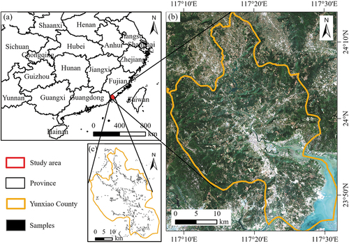
The study area is located in Yunxiao County, southeastern Fujian Province, China (Figure 1). This county has an area of 1054.3 km² and has a typical subtropical climate with an average annual temperature of 21.3°C and annual precipitation of 1730.6 mm. The terrain tilts from the southwest to the south, and the west, northeast, and southwest are mountainous, while the central and southeast are coastal alluvial plains (Figure 1(b)). The land covers in Yunxiao County are complex and fragmented due to the intense human activities in the past decades. The study area has a forest area of 40.1%, with a large proportion of eucalyptus plantations and economic forests. The fruit industry was well developed, with a large size of loquat, honey pomelo, and other subtropical fruit species. The famous Zhangjiangkou Mangrove National Nature Reserve is located at the mouth of the Zhang River in Yunxiao County.

Figure 1. Location of study area, Yunxiao County Fujian Province, China (a); a true color composite from Sentinel-2 data (b), and collected samples of vegetation types (c).

2.2. Datasets and data preprocessing

2.2.1. Sample data of vegetation types

The vegetation classification scheme was designed for ten categories considering their distribution and areal proportions. The names and sample information of these classes are summarized in Table 1. Field survey for collection of samples of vegetation types were conducted in July 2021. A total of 1301 samples (polygons) were collected. During the survey, each sample of vegetation types was drawn in the form of polygons based on the OvitalMap. Those polygons were overlaid on Sentinel-2 images with a spatial resolution of 10 m. The pixels within each polygon were extracted to build the dataset and input into classification models. We used five-fold cross-validation to evaluate the performance of different classification models by partitioning total samples (polygons) into five sets. Specifically, for each category, the sample polygons are divided equally into five parts (the polygon size of the same category in the survey data is similar). Four sets were used for training the models, and the remaining one set for evaluating the classification performance iteratively. The average accuracy of five results was regarded as the final accuracy of a particular classification model.

Table 1. Samples of different vegetation types.

Vegetation types	Number of polygons	Number of pixels
Eucalyptus plantation (EU)	334	10,099
Mangrove (MA)	96	839
Other broadleaf forest (OBL)	84	3337
Mixed broadleaf-conifer forest (MBC)	18	792
Loquat (LO)	92	923
Jujube (JU)	50	279
Honey pomelo (HP)	159	4176
Farmland (FA)	120	1462
Grassland (GR)	70	653
Non-vegetation (NV)	278	8665
Total	1301	31,225

2.2.2. Time series Sentinel-2 data and processes

A total of 63 Sentinel-2 L2A multispectral images with cloud coverage ratio less than 60%, covering the study area between January 2019 and July 2021, were collected from the Google Earth Engine platform (GEE) (Table 2). The bands with a spatial resolution of 20 m were resampled to 10 m using bilinear interpolation algorithm when exported at GEE. The percentage of valid values in the study area varied with a range between 27% and 98%. The contaminated pixels due to clouds and shadows were masked out based on the cloud probability band and filled using the SAMSTS method (L. Yan and Roy 2018). The time series data were then smoothed using the Savitzky-Golay filter (Schafer 2011). Previous studies have proven that data restoration followed by filter smoothing produced higher quality of time series data (Yan and Roy 2020). The time series dataset usually has unequal time intervals (Table 2). In order to generate equal-interval data, the spline interpolation method (Wolberg and Alfy 1999) was used to produce 8-day equal-interval time series data. The values generated by this method are consistent with the unequal-interval data, but with the time interval changed. Finally, a total of 114 values were obtained for each pixel through equal-interval interpolation. Both unequal and equal interval datasets were input into the classification models to examine the effect of interpolation on vegetation classification. Figure 2 exemplifies the time series of band 8 (near infrared), band 5 (red edge 1), and band 11 (shortwave infrared 1) in different processing stages for broadleaf forest.

Figure 2. Time series Sentinel-2 data of other broadleaf forest (OBL) in different spectral bands: (a) near-infrared (band 8), (b) red edge 1 (band 5), (c) shortwave infrared 1 (band 11).

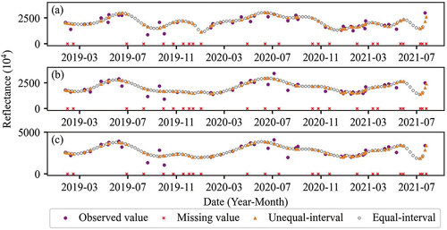
Table 2. Date distribution and valid value ratios of Sentinel-2 image used in this study.

Date	Ratio of valid value	Date	Ratio of valid value	Date	Ratio of valid value
24 January 2019	0.61	02 January 2020	0.82	01 January 2021	0.88
29 January 2019	0.55	27 January 2020	0.92	16 January 2021	0.93
06 February 2019	0.94	01 February 2020	0.89	21 January 2021	0.94
13 February 2019	0.39	21 February 2020	0.91	31 January 2021	0.94
13 March 2019	0.78	22 March 2020	0.72	05 February 2021	0.93
28 March 2019	0.39	13 April 2020	0.88	15 February 2021	0.96
24 April 2019	0.37	28 April 2020	0.89	20 February 2021	0.95
12 May 2019	0.91	06 May 2020	0.91	22 February 2021	0.94
14 May 2019	0.63	16 May 2020	0.27	12 March 2021	0.72
08 June 2019	0.87	12 June 2020	0.86	24 March 2021	0.56
16 June 2019	0.93	20 June 2020	0.55	11 April 2021	0.95
28 June 2019	0.42	05 July 2020	0.44	21 April 2021	0.97
10 August 2019	0.76	17 July 2020	0.3	11 May 2021	0.49
20 August 2019	0.41	09 August 2020	0.67	21 May 2021	0.55
19 September 2019	0.96	29 August 2020	0.72	28 May 2021	0.34
29 September 2019	0.9	03 September 2020	0.71	10 July 2021	0.47
01 October 2019	0.9	10 October 2020	0.88	15 July 2021	0.55
24 October 2019	0.86	25 October 2020	0.86	22 July 2021	0.64
03 November 2019	0.98	12 November 2020	0.94	25 July 2021	0.86
18 November 2019	0.85	22 November 2020	0.85
03 December 2019	0.87	22 December 2020	0.85
13 December 2019	0.96	27 December 2020	0.95

2.2.3. Time series Sentinel-2 data imaging

Recurrence plot is an effective method to analyze the periodicity and non-stationarity of time series data (Eckmann, Kamphorst, and Ruelle 1987). It calculates the similarity of different time trajectories. By transforming time series data into two-dimensional images, recurrence plot can better reveal the internal structure of time series (Eckmann, Kamphorst, and Ruelle 1987). Binary recurrence plot is a basic form of recurrence plots. It is determined by three parameters: embedding dimension (m), time delay ($\mathit{\tau }$), and threshold (r). Supposing a time series with length n is expressed as:

$\left(t_1,\mathit{\hspace{0.17em}}{t}_2,\mathit{\hspace{0.17em}}\dots ,\mathit{\hspace{0.17em}}{t}_{\mathit{n}-1},\mathit{\hspace{0.17em}}{t}_n\right)$

the trajectory of the $i^{\mathit{th}}$ time step is the vector ${\mathrm{T}}_i$, which can be expressed as:

$T_i=\left(t_i,\mathit{\hspace{0.17em}}{t}_{\mathit{i}+\mathit{\tau }},\dots \mathit{\hspace{0.17em}},\mathit{\hspace{0.17em}}{t}_{\mathit{i}+\left(\mathit{m}-1\right)\tau }\right),\mathit{\hspace{0.17em}}\mathit{i}\in 1,\mathit{\hspace{0.17em}}2,\mathit{\hspace{0.17em}}\dots ,\mathit{\hspace{0.17em}}\mathit{n}-\left(\mathit{m}-1\right)\mathit{\tau }$

where m represents the length of the trajectory, and $\mathit{\tau }$ represents the time interval between two observations (values). The recurrence plot is calculated by Equation (1)(1) ${\mathit{R}}_{\mathit{i},\mathit{\hspace{0.17em}}j}=\mathit{\hspace{0.17em}}\left\{\begin{array}{c}1,\left|\left|T_i-T_j\right|\right|\le \mathit{r}\\ 0,\left|\left|T_i-T_j\right|\right|>\mathit{r}\end{array}\right.$(1) .

(1) ${\mathit{R}}_{\mathit{i},\mathit{\hspace{0.17em}}j}=\mathit{\hspace{0.17em}}\left\{\begin{array}{c}1,\left|\left|T_i-T_j\right|\right|\le \mathit{r}\\ 0,\left|\left|T_i-T_j\right|\right|>\mathit{r}\end{array}\right.$(1)

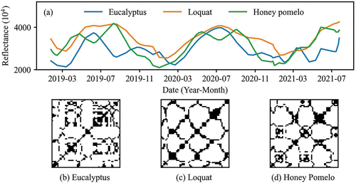
where r is a predefined threshold. The parameters m and $\mathit{\tau }$ were both set to 1 to examine the influence of paired observed values on vegetation classification. The threshold r determines the proportions of values 1 and 0 in the recurrence plot. It was supposed that the characteristics of time series can be accounted for by a small part of the time series (Eckmann, Kamphorst, and Ruelle 1987). The threshold r was set to 20% quantile of the trajectory distance, i.e. 20% of pixel values in the recurrence plot are 1, and other values are 0. Taking reflectance values of eucalyptus, loquat, and honey pomelo on near-infrared band in time series as examples, there are obvious differences in their recurrence plots (Figure 3).

Figure 3. Time series near-infrared reflectance (a) and corresponding recurrence plots for eucalyptus (b), loquat (c), and honey pomelo (d).

2.3. Classification models and performance evaluation

2.3.1. Classification models based on deep learning

Three classification models – CNN with 1DTS, GoogLeNet with recurrence plot data, and CGNet with both 1DTS and recurrence plot data were selected for vegetation classification based on Sentinel-2 time series data with unequal and equal intervals.

2.3.1.1 CNN with one-dimensional time series

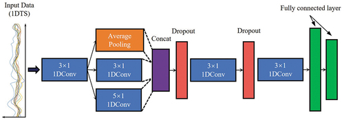
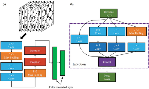
CNN uses convolution kernels to capture the unique patterns in the input data as features to support classification, regression, and other tasks (Rußwurm and Körner 2020). Conv1D uses multivariable time series as input and consists of several one-dimensional convolution, pooling, and dropout layers (Zhong, Hu, and Zhou 2019). Its receptive field gradually increases with the increase in the number of layers. The lower layers can capture local features of the time series, and the upper layers can capture more abstract and generalized semantic features (Zhong, Hu, and Zhou 2019). Finally classification was conducted through the fully connected layers. Here, we adopted the network structure of Conv1D to process the Sentinel-2 multi-band time series data (Figure 4). The fully connected layer was modified according to the number of vegetation classes.

Figure 4. The network structure of Conv1D. Concat operation concatenates the features from previous layers.

2.3.1.2 GoogLeNet with recurrence plot data

GoogLeNet is a type of CNN based on an inception architecture and takes images as input (Szegedy et al. 2015). It consists of several inception modules and has two advantages: 1) A 1 × 1 convolution is used to reduce dimensionality, and it extracts rich features and reduces computational complexity. 2) Convolution and aggregation are performed at multiple scales simultaneously, gathering multi-scale information and enriched features. Considering recurrence plot data from the time series Sentinel-2 dataset is not as complex as natural images, the GoogLeNet used here contains only a part of the blocks of the original architecture with some adjusted parameters (Figure 5). Ten time series Sentinel-2 bands for each pixel were transformed into recurrence plots using the method in Section 2.2.3 as input for this model.

Figure 5. Structure of GoogLeNet with recurrence plot data input (a), inception module used in GoogLeNet (b).

2.3.1.3 CGNet with one-dimensional time series and recurrence plot data

It is common to combine multi-source time series data for classification, regression, and forecasting tasks by using a model of multiple branches (Ienco et al. 2019; Interdonato et al. 2019). We designed a two-branch network (named CGNet) to integrate different data organizations (1DTS and recurrence plot). CGNet fully reuses the feature extractors of Conv1D and GoogLeNet, concatenates the features generated by these two networks, and adds a fully connected layer to process the high-dimensional features after concatenation. The parameters of Conv1D and GoogLeNet models were completely frozen during training, and only the parameters of the fully connected layer in the CGNet were updated.

2.3.2. Evaluation of model performances

F1 scores were used to explore the performance of deep learning classification methods. We further inspected the separability through t-SNE method and the distance of features vectors. We also examined the impacts of spectral and temporal features on classification.

2.3.2.1 F1 score

F1 scores were used to measure overall and each vegetation classification accuracies from different models. It is the harmonic mean of the producer’s and user’s accuracies. For each vegetation type, F1 is calculated by Equation (2)(2) $\mathrm{F}{1}_i=\frac{1}{\frac{1}{2}\left(\frac{1}{{\mathit{A}}_{\mathrm{producer}}}+\frac{1}{{\mathit{A}}_{\mathrm{use}r}}\right)}=\frac{2{\mathit{A}}_{\mathrm{producer}}\ast A_{\mathrm{user}}}{A_{\mathit{producer}}+A_{\mathrm{user}}}$(2) .

(2) $\mathrm{F}{1}_i=\frac{1}{\frac{1}{2}\left(\frac{1}{{\mathit{A}}_{\mathrm{producer}}}+\frac{1}{{\mathit{A}}_{\mathrm{use}r}}\right)}=\frac{2{\mathit{A}}_{\mathrm{producer}}\ast A_{\mathrm{user}}}{A_{\mathit{producer}}+A_{\mathrm{user}}}$(2)

where $\mathrm{F}{1}_i$ represents F1 score of vegetation type i, $A_{\mathit{producer}}$ and $A_{\mathit{user}}$ represent the producer’s and user’s accuracies of vegetation type i. The overall performance (F1) of a model was calculated by averaging all $\mathrm{F}{1}_i$. It means that all vegetation classes have the same weight on the models’ overall accuracy, and any poor recognition of a vegetation class will affect the overall performance of the classification model.

2.3.2.2 Separability analysis

The extracted features greatly affect the vegetation classification, and analysis of separability help us determine the best input data and network. Deep learning models can extract high-dimensional features from the input data, but directly analyzing the extracted features is challenging. To better visualize these features and their differences, 200 pixels were selected randomly for each category from all surveyed data. Each pixel comprises four types of features: Sentinel-2 spectral band, Conv1D, GoogLeNet, and CGNet. The Sentinel-2 spectral band feature is obtained by concatenating ten time series spectral bands with equal interval (8 days) produced in Section 2.2.2, and its dimension is 114 × 10. These time series datasets were input into the trained Conv1D and GoogLeNet, and their features with 512 dimensions were obtained respectively. By concatenating the Conv1D features and GoogLeNet features, the CGNet features with 512 × 2 dimensions were generated. The extracted features were processed using the t-SNE dimension reduction technique and then projected to a two-dimensional plane for better visualization (Hinton and Roweis 2002; Rußwurm and Körner 2020). For each type of features, the Euclidean Distances (ED) of feature vectors between all vegetation categories (each category has 200 feature vectors) were calculated and used to measure the separability (Equation (3)(3) $D_{\left(\mathit{e},\mathit{\hspace{0.17em}}g\right)}=\frac{1}{N^2}\sum _{\mathit{o}=1}^N\sum _{\mathit{p}=1}^N\mathit{ED}\left(V_o^e,\mathit{\hspace{0.17em}}{V}_p^g\right)$(3) ).

(3) $D_{\left(\mathit{e},\mathit{\hspace{0.17em}}g\right)}=\frac{1}{N^2}\sum _{\mathit{o}=1}^N\sum _{\mathit{p}=1}^N\mathit{ED}\left(V_o^e,\mathit{\hspace{0.17em}}{V}_p^g\right)$(3)

(4) $D_{\left(e,\hspace{0.17em}g\right)}^{\mathit{norm}}=\frac{{\mathit{D}}_{\left(\mathit{e},\mathit{\hspace{0.17em}}g\right)}-\min \left(\mathit{D}\right)}{max\left(\mathrm{D}\right)-\min \left(\mathrm{D}\right)}$(4)

where $D_{\left(\mathit{e},\mathit{\hspace{0.17em}}g\right)}$ is the ED between vegetation categories e and g, N is the number of feature vector (N = 200). $V_o^e$ and $V_p^g$ represent the $o^{\mathit{th}}\mathrm{and}\mathit{\hspace{0.17em}}{\mathrm{p}}^{\mathrm{th}}$ feature vectors in category e and g, respectively. Finally, the distances between all categories were normalized (the features distance matrix of each model is normalized separately) using Equation (4)(4) $D_{\left(e,\hspace{0.17em}g\right)}^{\mathit{norm}}=\frac{{\mathit{D}}_{\left(\mathit{e},\mathit{\hspace{0.17em}}g\right)}-\min \left(\mathit{D}\right)}{max\left(\mathrm{D}\right)-\min \left(\mathrm{D}\right)}$(4) . D represents the set of distances between all pairs of categories.

2.3.3. Importance analysis of spectral and temporal features for classification

A deep learning model can be considered a function that can fit any data and establish a map from the input domain X to the target domain Y. It can be expressed as $\mathit{Y}=\mathit{\hspace{0.17em}}{f}_{\theta }\left(\mathit{X}\right)$, where $\mathit{\theta }$ is parameter of the model and is iteratively optimized by applying the backpropagation algorithm together with the gradient descent. Gradients reflect the influence of these parameters on model performance. Similarly, we can calculate the gradients from the input data to analyze the importance of temporal and spectral features (Rußwurm and Körner 2020). We computed the gradient of the highest predicted score $\tilde{y}$ with respect to input data X. It can be described as:

(5) $\frac{\mathrm{\partial }\tilde{y}}{\mathrm{\partial X}}=\frac{\mathrm{\partial }\left[\max \left(f_{\theta }\left(\mathit{X}\right)\right)\right]}{\mathrm{\partial X}}\mathit{\hspace{0.17em}}$(5)

The gradient of input data reflects the influence of each input data element on the predicted results. Non-gradient indicates the relevant feature of input data has no or minimal impact on the prediction (low importance). The positive and negative gradients indicate that the change of corresponding features will affect the predicted score of this category. The larger magnitude of a gradient, the greater its importance. The importance of spectral and temporal features was quantified by calculating gradients of input time series. We focused on Conv1D and GoogLeNet models because CGNet is the combination of the two models. For Conv1D with 1DTS (ten bands) data as input, the importance of every time step was calculated. For GoogLeNet with recurrence plot as input, the importance of every paired time step was generated. In order to examine the importance of temporal dimension (IMT) to each vegetation class, the mean gradient of all samples (pixel level) of each class on every time step was calculated. The process of one class on one band can be described as Equations (6)(6) $\mathit{IM}{T}_{1\mathit{DTS}}=\left[{\bar{I}}_1,\mathit{\hspace{0.17em}}{\bar{I}}_2,\mathit{\hspace{0.17em}}\dots {\bar{I}}_{\mathit{n}-1},\mathit{\hspace{0.17em}}{\bar{I}}_{\mathit{n}}\right]$(6) and (7(7) $\mathit{IM}{T}_{\mathit{RP}}=\left[\begin{array}{ccc}{\bar{I}}_{\mathit{n},\mathit{\hspace{0.17em}}1}& \cdots & {\bar{I}}_{\mathit{n},\mathit{\hspace{0.17em}}\mathit{n}}\\ ⋮& \ddots & ⋮\\ {\bar{I}}_{1,\mathit{\hspace{0.17em}}1}& \cdots & {\bar{I}}_{1,\mathit{\hspace{0.17em}}\mathit{n}}\end{array}\right]$(7) ):

(6) $\mathit{IM}{T}_{1\mathit{DTS}}=\left[{\bar{I}}_1,\mathit{\hspace{0.17em}}{\bar{I}}_2,\mathit{\hspace{0.17em}}\dots {\bar{I}}_{\mathit{n}-1},\mathit{\hspace{0.17em}}{\bar{I}}_{\mathit{n}}\right]$(6)

where ${\bar{I}}_{\mathit{k}}=\frac{1}{\mathit{count}}\mathit{\hspace{0.17em}}{\sum }_{c=1}^{co\mathrm{unt}}{G}_s^c\left(\mathit{k}\right)$

(7) $\mathit{IM}{T}_{\mathit{RP}}=\left[\begin{array}{ccc}{\bar{I}}_{\mathit{n},\mathit{\hspace{0.17em}}1}& \cdots & {\bar{I}}_{\mathit{n},\mathit{\hspace{0.17em}}\mathit{n}}\\ ⋮& \ddots & ⋮\\ {\bar{I}}_{1,\mathit{\hspace{0.17em}}1}& \cdots & {\bar{I}}_{1,\mathit{\hspace{0.17em}}\mathit{n}}\end{array}\right]$(7)

where ${\bar{I}}_{\mathit{a},\mathit{\hspace{0.17em}}\mathit{b}}=\frac{1}{\mathit{count}}{\sum }_{c=1}^{co\mathrm{unt}}{G}_s^c\left(\mathit{a},\mathit{\hspace{0.17em}}\mathit{b}\right)$

n and $\mathit{\hspace{0.17em}}\bar{I}$ represent the length of time series and mean gradient of all pixel samples in a category respectively, count represents the number of all pixel samples in a category, and $G_s^c\left(\mathit{k}\right)$(or $G_s^c\left(\mathit{a},\mathit{\hspace{0.17em}}\mathit{b}\right)$) represents the gradient on $c^{\mathit{th}}$ pixel sample, band s, and position k (or a, b).

By using the method described above, we obtained the gradient of each time series element and the importance distribution in time series data. Similarly, we can also use absolute values of gradients (no matter positive or negative) to rank the band importance (IMB). This process can be expressed as Equations (8)(8) $\mathit{IMB}=\left[{\bar{B}}_1,\mathit{\hspace{0.17em}}{\bar{B}}_2,\mathit{\hspace{0.17em}}\dots ,\mathit{\hspace{0.17em}}{\bar{B}}_9,\mathit{\hspace{0.17em}}{\bar{B}}_{10}\right]$(8) –(10(10) ${\bar{B}}_{\mathit{s}}=\frac{1}{\mathit{count}\ast n\ast n}{\sum }_{c=1}^{co\mathrm{unt}}{\sum }_{a=1}^n{\sum }_{b=1}^n{G}_s^c\left(\mathrm{a},\mathrm{b}\right)$(10) ). The sorted IMB was used to obtain the importance rankings of bands.

(8) $\mathit{IMB}=\left[{\bar{B}}_1,\mathit{\hspace{0.17em}}{\bar{B}}_2,\mathit{\hspace{0.17em}}\dots ,\mathit{\hspace{0.17em}}{\bar{B}}_9,\mathit{\hspace{0.17em}}{\bar{B}}_{10}\right]$(8)

in Conv1D,

(9) ${\bar{B}}_{\mathit{s}}=\frac{1}{\mathit{count}\times n}{\sum }_{c=1}^{co\mathrm{unt}}{\sum }_{k=1}^n{G}_s^c\left(\mathit{k}\right)$(9)

in GoogLeNet,

(10) ${\bar{B}}_{\mathit{s}}=\frac{1}{\mathit{count}\ast n\ast n}{\sum }_{c=1}^{co\mathrm{unt}}{\sum }_{a=1}^n{\sum }_{b=1}^n{G}_s^c\left(\mathrm{a},\mathrm{b}\right)$(10)

Considering eucalyptus, loquat, and honey pomelo are very typical plantation and widely distributed in Yunxiao County. Thus, we chose these three vegetation types as representatives for spectral and temporal importance analysis.

3. Results

3.1. Comparative analysis of vegetation classification accuracy assessment

The equal-interval time series dataset significantly improved the accuracies of the overall classification and each vegetation type compared to the unequal-interval dataset (Figure 6 and Table 3). The most significant improvement was in the GoogLeNet model with F1 score increase of 0.13, followed by CGNet and Conv1D with F1 score increases of 0.09 and 0.04, respectively. The accuracy improvements for each vegetation category were various. The greatest improvement was for mixed broadleaf-conifer forest, whose F1 scores increased by 0.20–0.32, depending on the models. GoogLeNet was more sensitive to the interpolation than Conv1D. It performed worse than Conv1D in every category when using unequal-interval data. However, GoogLeNet outperformed Conv1D in most categories when using equal-interval time series as input data.

Figure 6. F1 scores of different models for unequal-interval and equal-interval time series data.

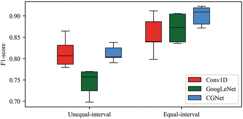
Table 3. F1 scores for each vegetation category and overall from different classification models.

Vegetation type	Unequal-interval			Equal-interval
	Conv1D	GoogLeNet	CGNet	Conv1D	GoogLeNet	CGNet
Eucalyptus plantation	0.93	0.87	0.91	0.93	0.94	0.96
Mangrove	0.96	0.91	0.95	0.95	0.95	0.98
Other broadleaf forest	0.62	0.50	0.59	0.60	0.70	0.73
Mixed broadleaf-conifer forest	0.41	0.36	0.39	0.61	0.66	0.71
Loquat	0.77	0.70	0.80	0.88	0.89	0.93
Jujube	0.82	0.80	0.82	0.85	0.88	0.90
Honey pomelo	0.95	0.94	0.96	0.98	0.99	0.99
Farmland	0.94	0.85	0.95	0.97	0.97	0.99
Grassland	0.78	0.58	0.78	0.82	0.79	0.86
Non-vegetation	0.96	0.94	0.97	0.96	0.96	0.96
Overall	0.81	0.74	0.81	0.85	0.87	0.90

The features of 1DTS from Conv1D and recurrence plot from GoogLeNet were mutually complementary in classification when the equal-interval time series was used. CGNet had the highest F1 score for most vegetation categories (Table 3) and the lowest variation (Figure 6) among three models. However, with unequal-interval time series data, the CGNet model only improved the accuracies of farmland, loquat, honey pomelo and non-vegetation slightly and performed equally or even worse than Conv1D for other vegetation types. The equal-interval time series data is crucial for fully using the information of 1DTS and recurrence plot. Therefore, the following analysis focused on the results from equal-interval data.

3.2. Separability analysis

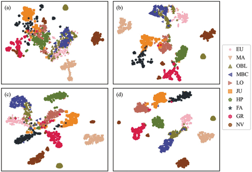
It is difficult to distinguish the main vegetation types from the original bands because the spectral information was highly mixed (Figure 7). The features extracted by the three models significantly improved their separabilities. For example, the spectral features of the mixed broadleaf-conifer forest, eucalyptus, and other broadleaf forest were interweaved in original bands, and so were the features of honey pomelo and loquat (Figure 7(a)). The features extracted by Conv1D and GoogLeNet had good discriminability for most vegetation categories. Honey pomelo and loquat can be distinguished well from other vegetation types (Figure 7(b,c)). The separabilities among mixed broadleaf-conifer forest, eucalyptus, and other broadleaf forest were further improved in the CGNet (Figure 7(d)).

Figure 7. Features visualization of (a) original bands, (b) Conv1D, (c) GoogLeNet, and (d) CGNet.

EU, eucalyptus plantation; MA, mangrove; OBL, other broadleaf forest; MBC, mixed broadleaf-conifer forest; LO, loquat; JU, jujube; HP, honey pomelo; FA, farmland; GR, grassland; and NV, non-vegetation.

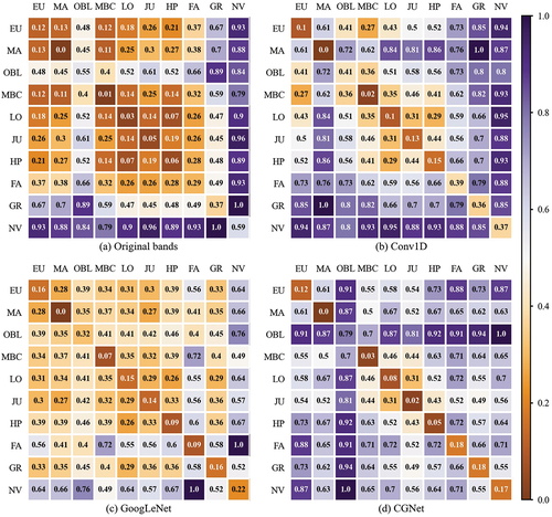
The separabilities expressed by distances between different categories in original data and the extracted features by three deep learning methods were very different (Figure 8). The inter-class distance between mixed broadleaf-conifer forests and eucalyptus was equal to the intra-class distance of eucalyptus (0.12) in original bands, implying the difficulties to be distinguished from each other. The intra-class distance of eucalyptus became smaller than the inter-class distance between mixed broadleaf-conifer forests and eucalyptus in Conv1D features. The intra-class distance of other broadleaf forest (0.55) was greater than the inter-class distance between eucalyptus and other broadleaf forest (0.48) in original bands, and this condition was improved by Conv1D feature (i.e. became 0.41 and 0.41, respectively). However, it was still difficult to distinguish these two types. GoogLeNet lessened this defect slightly with the intra-class distance smaller than the inter-class distance (0.32 and 0.39 respectively). CGNet improved the separability of all categories with intra-class distance smaller than 0.2 (except other broadleaf forest), and inter-class distance larger than 0.5 in almost all classes (Figure 8(d)). There are two clusters of broadleaf forest samples in Figure 7(a–d), indicating there are two very distinct broadleaf species in the study area. Compared with Conv1D and GoogLeNet, CGNet method amplified this phenomenon by a large intra-class distance of other broadleaf forest (0.79).

Figure 8. Distances between different vegetation categories in (a) original bands, (b) features of Conv1D, (c) features of GoogLeNet, and (d) features of CGNet.

EU, eucalyptus plantation; MA, mangrove; OBL, other broadleaf forest; MBC, mixed broadleaf-conifer forest; LO, loquat; JU, jujube; HP, honey pomelo; FA, farmland; GR, grassland; and NV, non-vegetation.

3.3. Importance of spectral and temporal features in different classification models

The gradients of eucalyptus, loquat, and honey pomelo in Conv1D were calculated for each Sentinel-2 band (Figure 9). The gradient curves of loquat and honey pomelo were obviously time-varying, while the curves of eucalyptus were more stable than other vegetation types. The gradient extremums were more concentrated in eucalyptus than in loquat and honey pomelo. The band importance rankings of three tree species were similar in Conv1D (Table 4). Band 5 (red edge 1) played an important role in distinguishing these vegetation types when using Conv1D features. The combination of band 5 and band 11 (short wave infrared 1) and the early period of the time series data (around October 2019) have the potential to differentiate eucalyptus from other vegetation classes. The first half year of the time series has a low contribution (i.e. the gradients in this time range are close to 0) for eucalyptus classification, which was quite different from that of loquat and honey pomelo. For loquat, two extremely low values of gradient curve on band 5 occurred around January 2020 and January 2021, and the gradient curves showed a periodic pattern and formed a stable period of high contribution after January 2020. More bands and time ranges had obvious extremum in gradient curves of honey pomelo.

Figure 9. Gradient curves of eucalyptus, loquat, and honey pomelo in Conv1D for ten spectral bands. (a) Eucalyptus, (b) Loquat, (c) Honey pomelo.

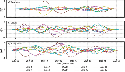
Table 4. Band importance rankings for eucalyptus, loquat, and honey pomelo in two models.

Ranking	Conv1D			GoogLeNet
	Eucalyptus	Loquat	Honey pomelo	Eucalyptus	Loquat	Honey pomelo
1	Band 5	Band 5	Band 5	Band 5	Band 5	Band 5
2	Band 11	Band 11	Band 11	Band 11	Band 4	Band 4
3	Band 2	Band 2	Band 3	Band 3	Band 12	Band 12
4	Band 3	Band 3	Band 2	Band 6	Band 2	Band 6
5	Band 12	Band 12	Band 12	Band 12	Band 6	Band 3
6	Band 6	Band 6	Band 6	Band 4	Band 3	Band 2
7	Band 4	Band 4	Band 8a	Band 2	Band 11	Band 11
8	Band 8a	Band 8a	Band 4	Band 8a	Band 7	Band 7
9	Band 7	Band 7	Band 7	Band 7	Band 8a	Band 8a
10	Band 8	Band 8	Band 8	Band 8	Band 8	Band 8

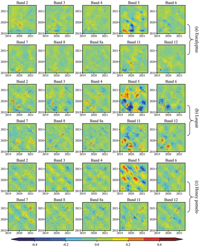
In GoogLeNet, the recognitions of eucalyptus, loquat, and honey pomelo were also strongly influenced by band 5. Band 4 (red) played a significant role in loquat and honey pomelo which was different from eucalyptus (also different from Conv1D) (Table 4). It indicated the features extracted by GoogLeNet were different from those in Conv1D. The gradient information presented from GoogLeNet was more complex than Conv1D (Figure 10). The gradient extremums of eucalyptus in recurrence plot were concentrated on the lower left corner of band 5, with the gradients reaching about −0.5 (Figure 10(a)). It indicates that the GoogLeNet paid more attention to the earlier part of the eucalyptus time series. The gradient distribution of recurrence plot in GoogLeNet on loquat and honey pomelo was similar to that in Conv1D; the gradient extremums were dispersive (especially in band 5).

Figure 10. Gradients distribution of recurrence plot in GoogLeNet for ten spectral bands. (a) Eucalyptus, (b) Loquat, (c) Honey pomelo.

3.4. Differences of vegetation classification results

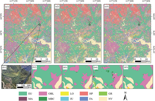
The three classification models showed different areal proportions of each category. Eucalyptus was the most widely distributed vegetation type, occupying about 37%−43% of the study area in different models. There was little difference in the spatial distribution of classification results among the three models (Figure 11(a1–a3)). GoogLeNet identified more eucalyptus in the northwest of the study area, while Conv1D and CGNet classified them as other broadleaf forest. Honey pomelo was distributed primarily in the north of the study area, while eucalyptus grew in the vast region outside the city. Other broadleaf forest was mainly distributed in the southwest mountains, and farmland was more distributed near the county center. Conv1D and GoogLeNet showed more fragmented results than those of CGNet from the local map view (Figure 11(b1–b5)).

Figure 11. Spatial distributions of vegetation types in the study area classified by Conv1D (a1), GoogLeNet (a2), and CGNet (a3). A local map of classification results: High-resolution drone image (b1), Visual interpretation (b2), Conv1D (b3), GoogLeNet (b4), CGNet (b5).

EU, eucalyptus plantation; MA, mangrove; OBL, other broadleaf forest; MBC, mixed broadleaf-conifer forest; LO, loquat; JU, jujube; HP, honey pomelo; FA, farmland; GR, grassland; and NV, non-vegetation.

3.5. Time cost

Despite attaining high accuracy in vegetation classification, deep learning possessed certain limitations. Deep learning is a computationally intensive method, and time efficiency is crucial, especially for remote-sensing big data (Zhang, et al. 2023). Deep learning methods generally need a large amount of data, their training time can often reach several hours or even several days. This study utilized the NVIDIA Quadro RTX 4000 8GB as the primary hardware for model training. Table 5 presents the training and prediction time incurred by different models and data formats. The training time of three models is less than one hour in both equal-interval and unequal-interval time series data. The Conv1D needs less time to predict, while GoogLeNet and CGNet take more time because images (i.e. recurrence plot) have a larger amount of data. It should be noted that the equal-interval data cost more time in the prediction stage. The final choice of the method and data preprocess depends on the requirements of the specific application.

Table 5. Time costs (hours) in different models and data.

Model	Unequal-interval		Equal-interval
	Training	Prediction	Training	Prediction
Conv1D	0.35	0.29	0.39	12.48
GoogLeNet	0.30	13.94	0.43	34.37
CGNet	0.66	14.38	0.69	34.32

4. Discussion

4.1. Effect of equal-interval time series interpolation on vegetation classification

The classification accuracies of three deep learning models were improved with the equal-interval time series data, indicating the necessity of equal-interval interpolation for time series data. Previous research found that interpolation had a significant impact on extraction of vegetation phenology information with obvious seasonal changes (e.g. deciduous broadleaf forest), but no significant effects on vegetation types without seasonal changes (such as evergreen broadleaf forests) (Li et al. 2021). However, our research showed that the interpolation operation had considerable accuracy improvement for almost all vegetation categories. The data with equal-interval used more time steps to describe the fluctuation of each time series curve, and the local variation of time series is amplified. This is beneficial for convolutional network, which needs multiple observations at adjacent times to capture the fluctuation information in the time series (Rußwurm and Körner 2020). In our experiment, the comparison between unequal and equal intervals bears similarities to the comparison between multi-temporal images and dense time series.

Previous studies have evaluated the effectiveness of dense time series data on land cover classification. For example, Zhong, Hu, and Zhou (2019) used deep learning and traditional machine learning methods to classify crops based on Landsat time series data as well as seasonality metrics. Their results showed that deep learning methods can better extract temporal features, and dense time series data contains rich surface information without the needs to add seasonality metrics. Xu et al. (2020) found that the classification accuracy increased by incorporating more observations of Landsat time series data, but there was an upper limit. Dense time series can provide more detailed seasonal features and short-term land cover change phenomena than multiple or single temporal data (Franklin et al. 2015; Zhu and Liu 2014). However, the improvement of classification accuracy in most studies has limitations, which might be because they used irregularly or available observations without interpolating the repaired data into equal time series data. In this study, we focused on the difference between equal-interval and unequal-interval data, which were both dense time series, showing that the features extracted from equal-interval data were more representative than those from unequal-interval data. This means that we can enhance the performance of dense time series in classification through equal-interval interpolation. Although the performance of equal-interval data is important, the essential difference between equal-interval and unequal-interval data is still unclear, and the mechanism by which equal-interval data improves model performance is also uncertain.

Equal-interval time series only increase the amount of data by mathematical interpolation and essentially do not enhance the surface spectral information. It may be that equal-interval data indirectly introduced temporal information which is critical for the model to extract time series features that can improve the classification results (Cai et al. 2018). Lattari, Rucci, and Matteucci (2022) added a module to deal with irregular time interval and achieved good results in time series feature extraction. The difference with our study is that they explicitly used data containing time interval information as part of the input data. So, explicit or implicit interval information is beneficial for time series feature extraction. Equal-interval data can also benefit the transferability of deep learning models. This is especially crucial in the case of optical sensor time series data, because the time interval in different regions is often uncertain due to data noises and cloudiness (Pasquarella et al. 2016; Tran et al. 2022; Vrieling et al. 2018).

4.2. Influence of time-series data organization forms on vegetation classification

Data organization forms impacted the performance of the deep learning-based classification model. Menini et al. (2018) employed recurrence plot and genetic programming to identify the eucalyptus regions and suggested that recurrence plot can obtain high classification accuracy using MODIS data. Our study showed recurrence plot had better performance with equal-interval time series Sentinel-2 data. In addition, we found that CGNet was able to significantly enhance the classification accuracy for most vegetation types by combining the features of 1DTS and recurrence plot. Specially, the improvement was more obvious for mixed broadleaf-conifer forest and classes with low accuracy in the recurrence plot-based model (GoogLeNet). It means 1DTS and recurrence plot are highly complementary to improve classification accuracy. Previous studies also proved the complementarity among other data organization forms, such as recurrence plot, Gramian angular field (GAF), and Markov transition field (MTF), when they were used as input data in the classification models (Dias, Dias, et al. 2020; Dias, Pinto, et al. 2020). Since all data organization forms are derived from the original time series, and no additional data is introduced, deep learning-based methods also need suitable feature extraction design before training the model.

Previous studies mainly focused on 2D-based data organization form, 1DTS and recurrence plot were rarely investigated. Recurrence plot contains static information about the correlation between all-time steps (every two values). 1DTS contains information about time series reflectance values and their trend. Each vegetation type has its unique reflectance fluctuation pattern (Gómez, White, and Wulder 2016; Rad et al. 2019; Senf et al. 2015), so this temporal information is crucial for classification. Dias, Dias, et al. (2020) proved that eucalyptus could be successfully classified even using only 2D representations, but they did not explore the performance of multi-category classification tasks (particularly with less variation between categories). Our study found that the 1DTS could further improve the performance of models with time series imaging data.

4.3. Importance of spectral and temporal features

Careful selection of appropriate time series data and spectral bands is crucial in remote sensing applications, particularly for vegetation classification. The gradients of input data and feature maps were commonly utilized to quantify feature importance. These methods can provide insights into the behavior of deep learning models and help guide data selection. Our study found that different vegetation types relied on different periods of data. Xu et al. (2020) employed a deep learning model to classify three crop types using time series data of various lengths, revealing that the optimal length of time series varied among different study subjects. Our study showed that the most critical spectral band was band 5 in the three deep learning models, but other important bands varied in different models and data formats. The temporal importance is also dependent on different vegetation types. Eucalyptus was focused on the early stage of the study period, while the important temporal ranges of loquat and honey pomelo were much scattered. This might be related to the growth characteristics and human disturbances. Eucalyptus was less disturbed than honey pomelo and loquat after it was planted, and the canopy closed after about two years. Loquat and honey pomelo may have different management measures (fertilization, weeding, density, trim, etc.), depending on their owners and terrain conditions. It should be noted that eucalyptus is a short-rotation plantation that is harvested often at 5–7 years old (Zhang et al. 2023). We did not distinguish the logging events because the next generation is regrown after a few months (D. Li et al. 2022). The logging events will be key information for eucalyptus classification for deep learning with long enough time series (Deng et al. 2020). The feature importance distribution on different categories can better assist us in selecting appropriate bands and dates of images to classify vegetation types.

4.4. Limitations of this study and potential solutions

Although deep learning methods often achieve better accuracy than traditional methods, the time cost of deep learning is also high, which is unfavorable for large-region mapping. The time cost of proposed methods may be influenced by various factors such as programming and computing platform (Dou et al. 2021). Nevertheless, there is room for enhancing efficiency and reducing the time required for training or forecasting. Firstly, there are only a few bands (such as band 5, band 11) that can fully capture the distinctive temporal characteristics of various categories. It is advisable to remove some bands with small contributions on classification to accelerate the speed of the network. Secondly, we can explore the use of a lightweight network, especially the GoogLeNet based on recurrence plot. The pixel values in recurrence plot are binary (1 or 0), which is not as complex and changeable as a raw image. Thus, reducing the network scale might have a positive effect on improving computational efficiency.

This study systematically evaluated the effectiveness of equal-interval time series and illustrated its advantages, which performed well in three deep learning models and different data organization forms (1DTS and recurrence plot). This means that we can use equal-interval interpolation to enhance the temporal feature of dense time series. Meanwhile, through quantitative research on the effect of 1DTS and recurrence plot, we found that the combination of two different data organization forms can improve the performance of equal-interval time series. There are also some limitations in this research. For example, it is unclear whether there exists an optimal time interval that can achieve the highest vegetation classification accuracy. This study used an 8-day interval, but did not test the impact of other time intervals. It is hard to explain the mechanism without detailed land surface observations. The complexity of land cover types might affect the performance of different deep learning methods. The roles of equal-interval time series and different data organization forms have not been effectively evaluated for different complex levels of vegetation types. In this study, we used Sentinel-2 time series imagery and focused only on temporal features for each pixel. The integration of spatial features and multi-sensor data (e.g. Sentinel-1 and Gaofen) could be beneficial for vegetation classification.

5. Conclusions

Based on unequal-interval and equal-interval time series Sentinel-2 data, we built 1DTS dataset and recurrence plot dataset, and used two convolutional networks (Conv1D, GoogLeNet) to classify the vegetation types in a subtropical area. We found that all models exhibited higher accuracy using equal-interval data than using unequal-interval data, and a significant improvement occurred using GoogLeNet. The features from 1DTS and recurrence plot were combined to construct CGNet. The classification accuracy was further improved, indicating that 1DTS and recurrence plot were complementary for fine vegetation classification. Band 5 (red edge 1) played as the first rank in the Conv1D and GoogLeNet models, but the order is very different in the three selected vegetation types in GoogLeNet model. The temporal importance also differed for the vegetation types in Conv1D and GoogLeNet models. Eucalyptus was a certain period, while loquat and honey pomelo showed more scattered importance distribution in the time series data. Recurrence plot contained additional information which was beneficial for fine vegetation classification, but the time cost should be considered in the large-scale application. This study provided a comprehensive evaluation of two data formats for Sentinel-2 data on fine vegetation classification and established a new network to integrate two kinds of extracted features.

Acknowledgments

The authors thank reviewers for their help to improve our manuscript.

Disclosure statement

No potential conflict of interest was reported by the author(s).

Additional information

Funding

This work was supported by National Key Research and Development Program of China [grant number 2021YFE0117700-2(2)], Natural Science Foundation of Fujian Province [grant number 2022J01640], Public Welfare Projects of Fujian Provincial Science and Technology Department [grant number 2021R1002008], National Natural Science Foundation of China [grant number 32371865], and the China Scholarship Council.

Notes on contributors

Ming Zhang

Ming Zhang is currently pursuing master degree at Fujian Normal University. His research interests are time series remote sensing and deep learning.

Dengqiu Li

Dengqiu Li received a PhD degree in Geography from Nanjing University. He is an associate professor at Fujian Normal University. His research interests include the classification of forest types and the monitoring of disturbances using dense time-series satellite remote sensing data and UAV Lidar. He specializes in evaluating the impacts of forest management and disturbances on the carbon cycle through the use of process-based ecosystem models and remote sensing data.

Guiying Li

Guiying Li received her PhD degree from Indiana State University and is an associate professor at Fujian Normal University. Her research interests are remote sensing, GIS, land use/cover change, and forestry.

Dengsheng Lu

Dengsheng Lu is currently a professor at School of Geographical Sciences, Fujian Normal University, Fuzhou, China. He graduated from Indiana State University in 2001, majoring in Physical Geography with a specialty in Remote Sensing and GIS. He had worked at Indiana University at Bloomington (2001–2006; 2008–2012), Auburn University (2007–2008), and Michigan State University (2012–2018). His research interests include remote sensing technologies and applications in tropical and subtropical forest ecosystems, in particular, in land use/cover change and forest biomass/volume estimation. In recent years, his research funds are mainly from the National Key R&D Program of China and NSFC. He has published 160+ articles with Google Scholar Citations of 27800 + . He was the “Most Cited Chinese Researchers” for the years 2019–2022. In the World’s Top 2% Scientists, he was also within the “career-long citation impact” in 2020–2023 and “citation impact during the single calendar year” in 2019–2022. He is an editorial board member in the journals such as International Journal of Digital Earth, Geo-Spatial Information Science, International Journal of Image and Data Fusion, Remote Sensing, and Frontiers in Remote Sensing.

References

- Brooks, E. B., V. A. Thomas, R. H. Wynne, and J. W. Coulston. 2012. “Fitting the Multitemporal Curve: A Fourier Series Approach to the Missing Data Problem in Remote Sensing Analysis.” IEEE Transactions on Geoscience & Remote Sensing 50 (9): 3340–3353. https://doi.org/10.1109/TGRS.2012.2183137.
- Cai, Y., K. Guan, P. Jian, S. Wang, C. Seifert, B. Wardlow, and L. Zhan. 2018. “A High-Performance and In-Season Classification System of Field-Level Crop Types Using Time-Series Landsat Data and a Machine Learning Approach.” Remote Sensing of Environment 210:35–47. https://doi.org/10.1016/j.rse.2018.02.045.
- Chelali, M., C. Kurtz, A. Puissant, and N. Vincent. 2021. “Deep-StaR: Classification of Image Time Series Based on Spatio-Temporal Representations.” Computer Vision and Image Understanding 208:103221. https://doi.org/10.1016/j.cviu.2021.103221.
- Deng, X., S. Guo, L. Sun, and J. Chen. 2020. “Identification of Short-Rotation Eucalyptus Plantation at Large Scale Using Multi-Satellite Imageries and Cloud Computing Platform.” Remote Sensing 12 (13): 2153. https://doi.org/10.3390/rs12132153.
- Dias, D., U. Dias, N. Menini, R. Lamparelli, G. L. Maire, and R. D. S. Torres. 2020. “Image-Based Time Series Representations for Pixelwise Eucalyptus Region Classification: A Comparative Study.” IEEE Geoscience & Remote Sensing Letters 17 (8): 1450–1454. https://doi.org/10.1109/LGRS.2019.2946951.
- Dias, D., A. Pinto, U. Dias, R. Lamparelli, G. L. Maire, and R. D. S. Torres. 2020. “A Multirepresentational Fusion of Time Series for Pixelwise Classification.” IEEE Journal of Selected Topics in Applied Earth Observations & Remote Sensing 13:4399–4409. https://doi.org/10.1109/JSTARS.2020.3012117.
- Dou, P., H. Shen, Z. Li, and X. Guan. 2021. “Time Series Remote Sensing Image Classification Framework Using Combination of Deep Learning and Multiple Classifiers System.” International Journal of Applied Earth Observation and Geoinformation 103 (1): 102477. https://doi.org/10.1016/j.jag.2021.102477.
- Eckmann, J. P., S. O. Kamphorst, and D. Ruelle. 1987. “Recurrence Plots of Dynamical Systems.” Europhysics Letters 4 (9): 973–977. https://doi.org/10.1209/0295-5075/4/9/004.
- Fang, F., B. E. McNeil, T. A. Warner, A. E. Maxwell, G. A. Dahle, E. Eutsler, and J. Li. 2020. “Discriminating Tree Species at Different Taxonomic Levels Using Multi-Temporal WorldView-3 Imagery in Washington D.C., USA.” Remote Sensing of Environment 246:111811. https://doi.org/10.1016/j.rse.2020.111811.
- Fawaz, H. I., G. Forestier, J. Weber, L. Idoumghar, and P. A. Muller. 2019. “Deep Learning for Time Series Classification: A Review.” Data Mining and Knowledge Discovery 33 (4): 917–963. https://doi.org/10.1007/s10618-019-00619-1.
- Franklin, S. E., O. S. Ahmed, M. A. Wulder, J. C. White, T. Hermosilla, and N. C. Coops. 2015. “Large Area Mapping of Annual Land Cover Dynamics Using Multitemporal Change Detection and Classification of Landsat Time Series Data.” Canadian Journal of Remote Sensing 41 (4): 293–314. https://doi.org/10.1080/07038992.2015.1089401.
- Gómez, C., J. C. White, and M. A. Wulder. 2016. “Optical Remotely Sensed Time Series Data for Land Cover Classification: A Review.” ISPRS Journal of Photogrammetry & Remote Sensing 116:55–72. https://doi.org/10.1016/j.isprsjprs.2016.03.008.
- Gong, P., H. Liu, M. Zhang, C. Li, J. Wang, H. Huang, N. Clinton, et al. 2019. “Stable Classification with Limited Sample: Transferring a 30-M Resolution Sample Set Collected in 2015 to Mapping 10-M Resolution Global Land Cover in 2017.” Science Bulletin 64 (6): 370–373. https://doi.org/10.1016/j.scib.2019.03.002.
- Gong, P., X. Li, J. Wang, Y. Bai, B. Chen, T. Hu, X. Liu, et al. 2020. “Annual Maps of Global Artificial Impervious Area (GAIA) Between 1985 and 2018.” Remote Sensing of Environment 236:111510. https://doi.org/10.1016/j.rse.2019.111510.
- Grings, F., E. Roitberg, and V. Barraza. 2019. “EVI Time-Series Breakpoint Detection Using Convolutional Networks for Online Deforestation Monitoring in Chaco Forest.” IEEE Transactions on Geoscience & Remote Sensing 58 (2): 1303–1312. https://doi.org/10.1109/TGRS.2019.2945719.
- Hakkenberg, C. R., M. P. Dannenberg, C. Song, and K. B. Ensor. 2019. “Characterizing Multi-Decadal, Annual Land Cover Change Dynamics in Houston, TX Based on Automated Classification of Landsat Imagery.” International Journal of Remote Sensing 40 (2): 693–718. https://doi.org/10.1080/01431161.2018.1516318.
- Hamida, A. B., A. Benoit, P. Lambert, and C. B. Amar. 2018. “3-D Deep Learning Approach for Remote Sensing Image Classification.” IEEE Transactions on Geoscience & Remote Sensing 56 (8): 4420–4434. https://doi.org/10.1109/TGRS.2018.2818945.
- Hinton, G. E., and S. Roweis. 2002. “Stochastic Neighbor Embedding.” In Proceedings of the 15th International Conference on Neural Information Processing Systems (NIPS), Cambridge, MA, 857–864. MIT Press. https://dl.acm.org/doi/10.5555/2968618.2968725.
- Huang, Z., L. Zhong, F. Zhao, J. Wu, H. Tang, Z. Lv, B. Xu, L. Zhou, R. Sun, and R. Meng. 2023. “A Spectral-Temporal Constrained Deep Learning Method for Tree Species Mapping of Plantation Forests Using Time Series Sentinel-2 Imagery.” ISPRS Journal of Photogrammetry & Remote Sensing 204:397–420. https://doi.org/10.1016/j.isprsjprs.2023.09.009.
- Ienco, D., R. Gaetano, C. Dupaquier, and P. Maurel. 2017. “Land Cover Classification via Multitemporal Spatial Data by Deep Recurrent Neural Networks.” IEEE Geoscience and Remote Sensing Letters 14 (10): 1685–1689. https://doi.org/10.1109/LGRS.2017.2728698.
- Ienco, D., R. Interdonato, R. Gaetano, and D. H. T. Minh. 2019. “Combining Sentinel-1 and Sentinel-2 Satellite Image Time Series for Land Cover Mapping via a Multi-Source Deep Learning Architecture.” ISPRS Journal of Photogrammetry & Remote Sensing 158:11–22. https://doi.org/10.1016/j.isprsjprs.2019.09.016.
- Interdonato, R., D. Ienco, R. Gaetano, and K. Ose. 2019. “DuPLO: A DUal View Point Deep Learning Architecture for Time Series Classification.” ISPRS Journal of Photogrammetry & Remote Sensing 149:91–104. https://doi.org/10.1016/j.isprsjprs.2019.01.011.
- Lattari, F., A. Rucci, and M. Matteucci. 2022. “A Deep Learning Approach for Change Points Detection in InSAR Time Series.” IEEE Transactions on Geoscience & Remote Sensing 60:1–16. https://doi.org/10.1109/TGRS.2022.3155969.
- Li, D., D. Lu, Y. Wu, and K. Luo. 2022. “Retrieval of Eucalyptus Planting History and Stand Age Using Random Localization Segmentation and Continuous Land-Cover Classification Based on Landsat Time-Series Data.” GIScience & Remote Sensing 59 (1): 1426–1445. https://doi.org/10.1080/15481603.2022.2118440.
- Li, X., W. Zhu, Z. Xie, P. Zhan, X. Huang, L. Sun, and Z. Duan. 2021. “Assessing the Effects of Time Interpolation of NDVI Composites on Phenology Trend Estimation.” Remote Sensing 13 (24): 5018. https://doi.org/10.3390/rs13245018.
- Menini, N., A. E. Almeida, R. Lamparelli, G. L. Maire, J. A. D. Santos, H. Pedrini, M. Hirota, and R. D. S. Torres. 2018. “A Soft Computing Framework for Image Classification Based on Recurrence Plots.” IEEE Geoscience & Remote Sensing Letters 16 (2): 320–324. https://doi.org/10.1109/LGRS.2018.2872132.
- Moskolaï, W. R., W. Abdou, and A. Dipanda. 2021. “Application of Deep Learning Architectures for Satellite Image Time Series Prediction: A Review.” Remote Sensing 13 (23): 4822. https://doi.org/10.3390/rs13234822.
- Pasquarella, V. J., C. E. Holden, L. Kaufman, and C. E. Woodcock. 2016. “From Imagery to Ecology: Leveraging Time Series of All Available Landsat Observations to Map and Monitor Ecosystem State and Dynamics.” Remote Sensing in Ecology and Conservation 2 (3): 152–170. https://doi.org/10.1002/rse2.24..
- Pelletier, C., G. I. Webb, and F. Petitjean. 2019. “Temporal Convolutional Neural Network for the Classification of Satellite Image Time Series.” Remote Sensing 11 (5): 523. https://doi.org/10.3390/rs11050523.
- Pringle, M. J., M. Schmidt, and J. S. Muir. 2009. “Geostatistical Interpolation of SLC-Off Landsat ETM+ Images.” ISPRS Journal of Photogrammetry & Remote Sensing 64 (6): 654–664. https://doi.org/10.1016/j.isprsjprs.2009.06.001.
- Rad, A. M., D. Ashourloo, H. S. Shahrabi, and H. Nematollahi. 2019. “Developing an Automatic Phenology-Based Algorithm for Rice Detection Using Sentinel-2 Time-Series Data.” IEEE Journal of Selected Topics in Applied Earth Observations & Remote Sensing 12 (5): 1471–1481. https://doi.org/10.1109/JSTARS.2019.2906684.
- Rußwurm, M., and M. Körner. 2020. “Self-Attention for Raw Optical Satellite Time Series Classification.” ISPRS Journal of Photogrammetry & Remote Sensing 169:421–435. https://doi.org/10.1016/j.isprsjprs.2020.06.006.
- Schafer, R. W. 2011. “What Is a Savitzky-Golay Filter?” IEEE Signal Processing Magazine 28 (4): 111–117. https://doi.org/10.1109/MSP.2011.941097.
- Sedukhin, S., Y. Tomioka, and K. Yamamoto. 2022. “In Search of the Performance-And Energy-Efficient CNN Accelerators.” IEICE Transactions on Electronics 105 (6): 209–221. https://doi.org/10.1587/transele.2021LHP0003.
- Senf, C., P. J. Leitão, D. Pflugmacher, S. V. D. Linden, and P. Hostert. 2015. “Mapping Land Cover in Complex Mediterranean Landscapes Using Landsat: Improved Classification Accuracies from Integrating Multi-Seasonal and Synthetic Imagery.” Remote Sensing of Environment 156:527–536. https://doi.org/10.1016/j.rse.2014.10.018.
- Shao, Y., and R. S. Lunetta. 2012. “Comparison of Support Vector Machine, Neural Network, and CART Algorithms for the Land-Cover Classification Using Limited Training Data Points.” ISPRS Journal of Photogrammetry & Remote Sensing 70:78–87. https://doi.org/10.1016/j.isprsjprs.2012.04.001.
- Shen, H., X. Li, Q. Cheng, C. Zeng, G. Yang, H. Li, and L. Zhang. 2015. “Missing Information Reconstruction of Remote Sensing Data: A Technical Review.” IEEE Geoscience and Remote Sensing Magazine 3 (3): 61–85. https://doi.org/10.1109/MGRS.2015.2441912.
- Szegedy, C., W. Liu, Y. Jia, P. Sermanet, S. Reed, D. Anguelov, D. Erhan, V. Vanhoucke, and A. Rabinovich. 2015. “Going Deeper with Convolutions.” In IEEE Conference on Computer Vision and Pattern Recognition (CVPR), Boston, MA, 1–9. Institute of Electrical and Electronics Engineers. https://doi.org/10.1109/CVPR.2015.7298594.
- Tan, Z., Z. Tan, J. Luo, and H. Duan. 2023. “Mapping 30-M Cotton Areas Based on an Automatic Sample Selection and Machine Learning Method Using Landsat and MODIS Images.” Geo-Spatial Information Science. Advance online publication. https://doi.org/10.1080/10095020.2023.2275622.
- Tarasiou, M., E. Chavez, and S. Zafeiriou. 2023. “ViTs for SITS: Vision Transformers for Satellite Image Time Series.” In 2023 IEEE/CVF Conference on Computer Vision and Pattern Recognition (CVPR), Vancouver, BC, Canada. Institute of Electrical and Electronics Engineers. https://doi.org/10.1109/CVPR52729.2023.01004.
- Tariq, A., J. Yan, A. S. Gagnon, M. R. Khan, and F. Mumtaz. 2023. “Mapping of Cropland, Cropping Patterns and Crop Types by Combining Optical Remote Sensing Images with Decision Tree Classifier and Random Forest.” Geo-Spatial Information Science 26 (3): 302–320. https://doi.org/10.1080/10095020.2022.2100287.
- Thiel, M., M. C. Romano, and J. Kurths. 2004. “How Much Information Is Contained in a Recurrence Plot?” Physics Letters: A 330 (5): 343–349. https://doi.org/10.1016/j.physleta.2004.07.050.
- Torre, D. M. G. D., J. Gao, C. Macinnis-Ng, and Y. Shi. 2021. “Phenology-Based Delineation of Irrigated and Rain-Fed Paddy Fields with Sentinel-2 Imagery in Google Earth Engine.” Geo-Spatial Information Science 24 (4): 695–710. https://doi.org/10.1080/10095020.2021.1984183.
- Tran, K. H., X. Zhang, A. R. Ketchpaw, J. Wang, Y. Ye, and Y. Shen. 2022. “A Novel Algorithm for the Generation of Gap-Free Time Series by Fusing Harmonized Landsat 8 and Sentinel-2 Observations with PhenoCam Time Series for Detecting Land Surface Phenology.” Remote Sensing of Environment 282:113275. https://doi.org/10.1016/j.rse.2022.113275.
- Turkoglu, M. O., S. D’Aronco, G. Perich, F. Liebisch, C. Streit, K. Schindler, and J. D. Wegner. 2021. “Crop Mapping from Image Time Series: Deep Learning with Multi-Scale Label Hierarchies.” Remote Sensing of Environment 264:112603. https://doi.org/10.1016/j.rse.2021.112603.
- Vrieling, A., M. Meroni, R. Darvishzadeh, A. K. Skidmore, T. Wang, R. Zurita-Milla, K. Oosterbeek, B. O’Connor, and M. Paganini. 2018. “Vegetation Phenology from Sentinel-2 and Field Cameras for a Dutch Barrier Island.” Remote Sensing of Environment 215:517–529. https://doi.org/10.1016/j.rse.2018.03.014.
- Weerakody, P. B., K. W. Wong, G. Wang, and W. Ela. 2021. “A Review of Irregular Time Series Data Handling with Gated Recurrent Neural Networks.” Neurocomputing 441:161–178. https://doi.org/10.1016/j.neucom.2021.02.046.
- Wen, Q., T. Zhou, C. Zhang, W. Chen, Z. Ma, J. Yan, and L. Sun. 2023. “Transformers in Time Series: A Survey.” In Proceedings of the Thirty-Second International Joint Conference on Artificial Intelligence (IJCAI), Macao, P.R. China, 6778–6786. Morgan Kaufmann. https://doi.org/10.24963/ijcai.2023/759.
- White, M. A., K. Beurs, K. Didan, D. W. Inouye, and O. P. Jensen. 2009. “Intercomparison, Interpretation, and Assessment of Spring Phenology in North America Estimated from Remote Sensing for 1982–2006.” Global Change Biology 15 (10): 2335–2359. https://doi.org/10.1111/j.1365-2486.2009.01910.x.
- Wolberg, G., and I. Alfy. 1999. “Monotonic Cubic Spline Interpolation.” In Proceedings Computer Graphics International, Canmore, Canada, 188–195. Institute of Electrical and Electronics Engineers. https://doi.org/10.1109/CGI.1999.777953.
- Wulder, M. A., D. P. Roy, V. C. Radeloff, T. R. Loveland, M. C. Anderson, D. M. Johnson, S. Healey, et al. 2022. “Fifty Years of Landsat Science and Impacts.” Remote Sensing of Environment 280:113195. https://doi.org/10.1016/j.rse.2022.113195.
- Xiao, C., E. Choi, and J. Sun. 2018. “Opportunities and Challenges in Developing Deep Learning Models Using Electronic Health Records Data: A Systematic Review.” Journal of the American Medical Informatics Association 25 (10): 1419–1428. https://doi.org/10.1093/jamia/ocy068.
- Xu, J. F., Y. Zhu, R. H. Zhong, Z. X. Lin, J. L. Xu, H. Jiang, J. F. Huang, H. F. Li, and T. Lin. 2020. “DeepCropmapping: A Multi-Temporal Deep Learning Approach with Improved Spatial Generalizability for Dynamic Corn and Soybean Mapping.” Remote Sensing of Environment 247:111946. https://doi.org/10.1016/j.rse.2020.111946.
- Yan, J., J. Liu, L. Wang, D. Liang, Q. Cao, W. Zhang, and J. Peng. 2022. “Land-Cover Classification with Time-Series Remote Sensing Images by Complete Extraction of Multiscale Timing Dependence.” IEEE Journal of Selected Topics in Applied Earth Observations & Remote Sensing 15:1953–1967. https://doi.org/10.1109/JSTARS.2022.3150430.
- Yan, L., and D. P. Roy. 2018. “Large-Area Gap Filling of Landsat Reflectance Time Series by Spectral-Angle-Mapper Based Spatio-Temporal Similarity (SAMSTS).” Remote Sensing 10 (4): 609. https://doi.org/10.3390/rs10040609.
- Yan, L., and D. P. Roy. 2020. “Spatially and Temporally Complete Landsat Reflectance Time Series Modelling: The Fill-And-Fit Approach.” Remote Sensing of Environment 241:111718. https://doi.org/10.1016/j.rse.2020.111718.
- Yan, J., L. Wang, H. He, D. Liang, W. Song, and W. Han. 2022. “Large-Area Land-Cover Changes Monitoring with Time-Series Remote Sensing Images Using Transferable Deep Models.” IEEE Transactions on Geoscience & Remote Sensing 60:1–17. https://doi.org/10.1109/TGRS.2022.3160617.
- Yuan, Y., and L. Lin. 2020. “Self-Supervised Pretraining of Transformers for Satellite Image Time Series Classification.” IEEE Journal of Selected Topics in Applied Earth Observations & Remote Sensing 14:474–487. https://doi.org/10.1109/JSTARS.2020.3036602.
- Yuan, Y., L. Lin, Q. Liu, R. Hang, and Z. G. Zhou. 2022. “SITS-Former: A Pre-Trained Spatio-Spectral-Temporal Representation Model for Sentinel-2 Time Series Classification.” International Journal of Applied Earth Observation and Geoinformation 106:102651. https://doi.org/10.1016/j.jag.2021.102651.
- Yu, X., J. Pan, M. Wang, and J. Xu. 2023. “A Curvature-Driven Cloud Removal Method for Remote Sensing Images.” Geo-Spatial Information Science 25 (2): 278–294. https://doi.org/10.1080/10095020.2023.2189462.
- Zhang, X., L. Liu, T. Zhao, X. Chen, S. Lin, J. Wang, J. Mi, and W. Liu. 2023. “GWL_FCS30: A Global 30 M Wetland Map with a Fine Classification System Using Multi-Sourced and Time-Series Remote Sensing Imagery in 2020.” Earth System Science Data 15 (1): 265–293. https://doi.org/10.5194/essd-15-265-2023.
- Zhang, Y., D. Lu, X. Jiang, Y. Li, and D. Li. 2023. “Forest Structure Simulation of Eucalyptus Plantation Using Remote-Sensing-Based Forest Age Data and 3-PG Model.” Remote Sensing 15 (1): 183. https://doi.org/10.3390/rs15010183.
- Zhang, Z., M. Zhang, J. Gong, X. Hu, H. Xiong, H. Zhou, and Z. Cao. 2023. “LuoJiaAI: A Cloud-Based Artificial Intelligence Platform for Remote Sensing Image Interpretation.” Geo-Spatial Information Science 26 (2): 218–241. https://doi.org/10.1080/10095020.2022.2162980.
- Zhong, L., L. Hu, and H. Zhou. 2019. “Deep Learning Based Multi-Temporal Crop Classification.” Remote Sensing of Environment 221:430–443. https://doi.org/10.1016/j.rse.2018.11.032.
- Zhu, X., and D. Liu. 2014. “Accurate Mapping of Forest Types Using Dense Seasonal Landsat Time-Series.” ISPRS Journal of Photogrammetry & Remote Sensing 96:1–11. https://doi.org/10.1016/j.isprsjprs.2014.06.012.
- Zhu, Z., M. A. Wulder, D. P. Roy, C. E. Woodcock, M. C. Hansen, V. C. Radeloff, S. P. Healey, et al. 2019. “Benefits of the Free and Open Landsat Data Policy.” Remote Sensing of Environment 224:382–385. https://doi.org/10.1016/j.rse.2019.02.016.