Assessing the consistency and reliability of the line intercept transect method in coral cover estimation using structure from motion photogrammetry techniques

Abstract

Appropriate coral reef monitoring methods and descriptors determine the effectiveness of ecosystem status assessment. We combined line intercept transect (LIT) and SfM technologies for image acquisition, and the POS information of images is defined and assigned in the relative coordinate system we build. Then, constructed high-resolution orthomosaics of coral reefs along measuring tapes in Metashape. We compared the estimates of coral cover by three methodologies (LIT, LIT on orthomosaic (LITO), surface analyses on orthomosaic (SAO)) and used virtual transects on orthomosaics and their estimates of coral cover to assess the consistency and reliability of LIT. The results show that the estimation of coral cover by LITO or LIT is more consistent and reliable when coral cover is higher, and the probability of overestimation is lower. SfM technology is increasingly used in coral reef survey and assessment, and has the potential to become the new standard for coral reef survey.

Keywords:

• Coral reefs
• underwater photogrammetry
• line intercept transect
• structure from motion
• coral cover

1. Introduction

Coral reef ecosystems are complex seafloor geomorphic systems (Hoegh-Guldberg, et al. 2007; Leon et al. 2015). Scleractinian corals, as the main producer of the carbonate framework (Chave et al. 1972), play the most important role in the formation of coral reefs. Coral reefs not only provide food and shelter for many reef-dwelling organisms (Stella et al. 2011; Brandl et al. 2018) but also have great tourism, leisure and economic value (Hoegh-Guldberg et al. 2007). In addition, reef structural complexity modifies wave processes, which have important forcing functions on shallow reefs as they act upon the majority of ecological and biogeochemical processes by exerting direct physical stress, indirectly mixing water (temperature and nutrients) and transporting sediments, nutrients and plankton (Hearn 2011). However, in recent decades, anthropogenic threats (rising ocean temperatures and declining ocean pH) (Gardner et al. 2003; Bellwood et al. 2004; Hughes et al. 2017) and the increased frequency of crown-of-thorns starfish outbreaks have reduced global coral cover, reef complexity and reef accretion potential (Alvarez-Filip et al. 2009; Perry et al. 2018). For example, human impacts and climate change effects have led to a massive decline in coral reef complexity in the Caribbean and Indo-Pacific (Hoegh-Guldberg et al. 2007; Perry et al. 2018; Carlot et al. 2020). Coral mass mortality caused by coral bleaching events has become more frequent in major coral reefs around the world, attracting global attention (Heron et al. 2016; Hughes et al. 2017). Plastic pollution is an emerging threat to coral reefs, spreading throughout reef food webs (Santos et al. 2021) and increasing disease transmission and structural damage to reef organisms (Lamb et al. 2018). And the latest research results show that plastics or other anthropogenic debris were found in some of Earth’s most remote and near-pristine reefs, such as in uninhabited central Pacific atolls (Pinheiro et al. 2023). At the same time, many international efforts and attempts to protect coral reef ecosystems are underway and conservation and management strategies for coral reefs continue to be proposed (e.g. the latest research results reveal that enhanced integrated land–sea management could help achieve coastal ocean conservation goals and provide coral reefs with the best opportunity to persist in our changing climate (Gove et al. 2023)).

Monitoring methods and tracking coral reef descriptors contribute to depictions of the state and changes of coral reefs. This is critical for understanding their future status under climate change, ecological disasters or other anthropogenic stress scenarios and to assess their potential recovery from these impacts (Hedley et al. 2016). Appropriate monitoring methods and descriptors not only determine the effectiveness of coral reef ecosystem status assessments (Urbina-Barreto et al. 2021b), but also serve as the basis for scientific research, conservation measures and ecological restoration decisions regarding coral reef ecosystems. The line intercept transect (LIT) method, a small-scale underwater field survey method, is widely used because it is relatively easy and inexpensive and is well suited to obtaining long-term monitoring data for reef benthic communities and assessing coral cover (Hill and Wilkinson 2004). It is also recommended by the Global Coral Reef Monitoring Network (GCRMN) (Hill and Wilkinson 2004). Remote sensing techniques can characterize the morphology and distribution of coral reefs at medium–large scales. A number of studies have successfully used traditional remote sensing techniques (airborne or satellite-mounted multispectral or hyperspectral devices) (Hochberg et al. 2003; Joyce and Phinn 2013; Joyce et al. 2013; Hedley et al. 2016) to map coral cover by interpreting spectral information. However, in practice, due to the limitations of water depth and transparency, traditional remote sensing techniques are not suitable for all coral reef distribution areas. The monitoring accuracy is also limited by spectral variability in benthic species and large-scale mixing at subpixel resolutions (Knudby et al. 2007; Hedley et al. 2012).

A number of new coral reef descriptors and novel coral reef monitoring methods have emerged that improve the quantity and quality of data to better understand coral reef ecosystems (Elise et al. 2019; Lechene et al. 2019; Zawada et al. 2019; Urbina-Barreto et al. 2021a). For example, high-spatial resolution bathymetric LiDAR (Goodman et al. 2020; Le Quilleuc et al. 2021), autonomous underwater vehicles (AUVs) (Friedman et al. 2012; Modasshir and Rekleitis 2020; Antervedi et al. 2021; Zhou et al. 2022), echo sounders or multibeam technologies (Bejarano et al. 2011; Abadie et al. 2018; Czechowska et al. 2020; Muhamad et al. 2023), consumer-grade unmanned aerial vehicles (UAVs) (Casella et al. 2017; Fallati et al. 2020; Giles et al. 2023) can produce high-resolution digital terrain models (DTMs), bathymetric surveys or high-resolution coral reef maps from which multiscale measures of roughness, slope and aspect can be derived.

The method adopted in this article is underwater photogrammetry (Bythell et al. 2001) using the structure from motion (SfM) technique (Burns et al. 2015; Nocerino et al. 2020), which can generate a 3D model of coral reefs, Digital Terrain Model (DTM), point clouds and orthomosaics (Westoby et al. 2012; McCarthy and Benjamin 2014; Ferrari et al. 2016; Palma et al. 2017; Urbina-Barreto et al. 2021b; Montalbetti et al. 2022) and reproduce small areas at a significant scale (Anelli et al. 2019). Photogrammetry is cost-effective (Burns et al. 2015) and noninvasive (Westoby et al. 2012; Lange and Perry 2020), allowing us to take objective measurements of the structure and complexity of coral reefs, which provide insights into benthic communities and their temporal changes (Nocerino et al. 2020). Specific applications include quantifying a series of structural complexity parameters (Anelli et al. 2019; Bayley et al. 2019), quantifying growth rates (changes in height or volume) for different coral species (Bennecke et al. 2016; Ferrari et al. 2017; Neyer et al. 2018; Bayley 2019; Rossi et al. 2020), tracking changes in colony morphology over time (Burns et al. 2015; Lavy et al. 2015) and assessing ecosystem function (Storlazzi et al. 2016).

In this study, SfM technique was used to construct high-resolution orthomosaics for analysing coral recruitment distribution. We compared the estimates of percent coral cover generated by the three methods: traditional LIT, LIT on orthomosaic (LITO) and surface analyses on orthomosaic (SAO). Taking estimates of coral cover by SAO as the reference, we analysed the reliability and consistency of coral cover estimations by LITO under different percentages of coral cover (ranging from a low percentage to over 50%).

2. Materials and methods

2.1. Study sites

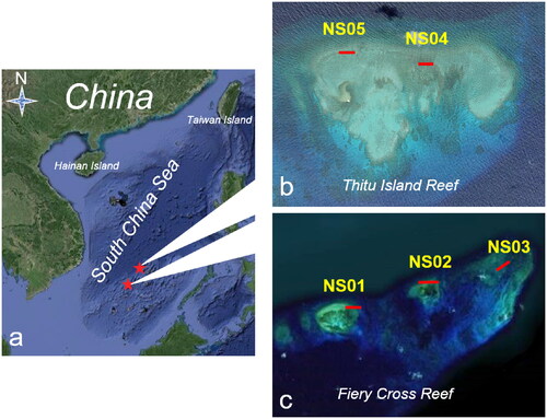
The study area is located in China’s Nansha Islands in the South China Sea, as shown in Figure 1(a). The five sites within the study area have different coral coverages. Sites NS01, NS02 and NS03 are located to the northwest of Fiery Cross Reef (Figure 1(c)), while NS04 and NS05 are located to the west of Thitu Island (Figure 1(b)). The topographies of the five sites consist of reef flats or outer reef slopes with water depths of 5 to 10 m. The substrate is dominated by reefs containing hard corals and a few other reef organisms. Hard corals are mainly massive corals (Porites spp., Lobophyllia spp., Favites spp., Favia spp., Goniastrea spp.), branching/corymbose corals (Acropora spp., Pocillopora spp.), encrusting corals (Montipora spp., Pavona spp.) and a few individual corals (Fungia spp.). Other reef organisms mainly include soft corals (mainly Sarcophyton spp.), macrobenthic algae (Mainly Dictyosphaeria versluysii), gorgonians, ascideans and sponges.

Figure 1. Study area and surveyed reefs. NS01, NS02 and NS03 located on Fiery Cross Reef, NS04 and NS05 located on Thitu Island Reef. The red lines represent approximately the position of the transects.

2.2. Image acquisition

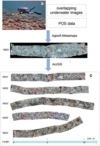
In May 2020, LIT surveys combined with SfM techniques were used for image acquisition. Ten meters measuring tape was placed parallel to the reef isobath, 0–15 cm above the bottom (Hill and Wilkinson 2004), as shown in Figure 2(a). The complex reef structures helped stabilize the transect line and kept it taut to minimize the bowing caused by the current. The SCUBA operator swam along the transect at a low speed and took consecutive vertically oriented images of the seafloor while maintaining a consistent height above the bottom. Take every photo manually and use the scale segments of measuring tape in adjacent images to ensure the overlap. To ensure that the scale on the measuring tape can be clearly read, we set the height to about 1 m. Each transect was photographed in three passes while ensuring that image overlap exceeded 80% in both the horizontal and along-track directions. The camera used was a Canon PowerShot G1 X Mark III, with an underwater case and the following specifications: sensor CMOS 23.7 mm × 15.6 mm, 6000 × 4000 pixels, focal length 15 mm.

Figure 2. Workflow of methods used to derive the orthomosaics using SfM and subsequent analysis. (a) Laying a transect with the measuring tape and acquiring overlapping images and POS data. (b) Using the Agisoft Metashape to process the images and POS data and to generate orthomosaics of each transect. (c) Orthomosaics of five transects after buffering analysis within ArcGIS.

2.3. Data processing

2.3.1. Position and orientation system data

Position and orientation system (POS) data, when used as the initial input for image position and attitude information in subsequent processing, can increase the speed of software processing and improve the quality of the results (Leon et al. 2015). On land, POS data can be easily obtained from the camera’s own system (GPS information stored directly in Exif imagery metadata) or with additional equipment. However, POS data can be difficult to obtain underwater due to the absence of satellite signals and the high cost of carrying underwater attitude and position sensors. Other underwater coral reef photogrammetry studies employed a variety of simple methods to synchronize positions acquired on the surface to those underwater. For example, the average distance between adjacent images was calculated based on the number of images and the length of the transect, and the GPS coordinates of each photo were estimated based on the GPS coordinates of the starting and ending points of the transect (Leon et al. 2015); SCUBA operators towed a locator buoy while capturing underwater images, and then, calculated the image coordinates by matching time to convert the coordinates (Palma et al. 2017). Since this study does not need the actual underwater geographic location information, only the relative image coordinates are used as the POS data. We use the idea of the first method above to calculate the relative image coordinates, and the specific steps are as follows: the first image of each transect was used as the reference point and the position coordinates of that image become the origin of the relative coordinate system; the Z axis was defined as the vertical direction perpendicular to the seafloor, the Y-axis was defined as the along-transect direction and positive and negative axes were defined following the right-handed Cartesian coordinate system; then, according to the length of the transect and the number of images, the relative coordinates of each photo were evenly interpolated.

2.3.2. Orthomosaic and scale

We used the Agisoft Metashape Pro (v1.8.5) to build orthomosaics of each transect. The principal processing steps are as follows: aerial triangulation, optimization, dense surface reconstruction and orthomosaic generation (Leon et al. 2015), and the specific processing workflow and parameters in Metashape are shown in Table 1. Due to Metashape’s built-in proprietary algorithm and by setting the camera to a narrow field of view (to reduce image distortion) (Young et al. 2017), we can obtain orthomosaics with millimetre resolution (Figure 2(b)). Then, orthomosaics were processed manually within ArcGIS (ArcMap 10.5). A buffer analysis with ArcGIS geo-processing tools was performed on both sides of the measuring tape (as the baseline) to obtain a new orthomosaic (Figure 2(c)), and the buffer distance of the five orthomosaics is uniformly set as 0.5 m, which can ensure that the information in the buffer area is clear and complete for all five transects. The coordinates in Orthomosaics are determined only by the POS information, so the accuracy is low. Therefore, the measuring tape visible within the orthomosaics was used to provide reference. The measuring tape segments with clear scales and minimal deformations were extracted as references in Metashape; the length of each reference scale segment was 0.1 m, and each transect contained 10 reference scale segments evenly distributed throughout the whole transect. Finally, the scaling factor was calculated as a correction factor for subsequent statistical analysis in ArcGIS. (1) $$\text{Scaling factor}=\frac{\sum _{i=1}^{10}\mathit{\text{Li}}}{10\times L0}$$(1) where Li is the length on the orthomosaic of each reference scale segment, and L0 is 0.1 m.

Table 1. Processing workflow and parameters in Metashape.

Processing workflow	Parameters
Add photos	–
Import reference	–
Align photos	Accuracy: High Generic preselection: Yes Reference preselection: Source
Build model	Surface type: Arbitrary Source data: Depth maps Interpolation: Enabled Quality: High Filtering mode: Disabled
Build texture	Texture: Diffuse map Source data: Images Mapping mode: Adaptive orthophoto Blending mode: Mosaic Enable hole filling: Yes Enable ghosting filter: Yes
Build orthomosaic	Projection type: Geographic (Local Coordinates (m)) Surface: Model Blending mode: Mosaic Refine seamlines: Yes Enable hole filling: Yes

2.3.3. Coral cover estimation

coral recruits can reflect the structural composition and future growth trend of coral communities, and are an important part of estimating coral cover. At present, there is no uniform definition of coral recruits, and most scholars take the maximum diameter as the discriminant index (Edmunds 2000; Hill and Wilkinson 2004; Birrell et al. 2008; Penin et al. 2010; Adjeroud et al. 2018; Liao 2021). In this study, the threshold value is 3.14 cm² (approximately equal to the area of a circle with a diameter of 2 cm); that is, corals with areas less than the threshold were considered coral recruits.

Three methods were used to estimate coral cover: LIT, LITO and SAO. LIT used to require SCUBA divers to do all the work on site: move slowly along the transect recording the growth forms (species if possible) directly under the tape; record the transition point on the tape (in cms) where the organism, substrate, growth form changes (Hill and Wilkinson 2004); estimate the percent coral coverage by dividing the number of points with live coral by the total number of points in the transect. However, we only recorded video on site and went back indoors to complete the statistics, recording only the coral cover, not the growth forms. The percent coral cover by LITO is estimated by dividing the total length that measuring tape intersected corals by the length of the measuring tape in the orthomosaic. In addition, we set up some virtual transects parallel to the tape measure on the orthomosaic and calculated coral cover estimation of the virtual transects using the LITO method in ArcGIS. Coral cover estimation calculated by SAO involves the following two steps: First, all coral colonies on the orthomosaic analyzed by buffer were extracted (trace polygons around the coral colonies by hand and calculate the planar area of those polygons in ArcGIS); finally, the ratio of the total planar area of all coral colonies to the orthomosaic area was the coral cover estimation of SAO.

3. Results

Some of the image acquisition and data processing results are shown in Table 2. A total of 808 images were acquired along the five transects, and the number of images in each transect ranged from 120 to 180. The pixel resolutions of the orthomosaics range from 0.15 mm to 0.36 mm. The reason for the discrepancy is that the divers cannot maintain a constant height above the sea floor when taking images because of issues of waves and the uneven ocean floor. The closer the distance to the seabed, the narrower field of view and the higher the resolution of the imagery. According to the pixel resolutions of the orthomosaics and camera parameters, the average photography height of each station can be calculated. It can be seen from Table 2 that the average photography height of NS02 is the lowest, 0.58 m; NS05 has the highest average photography height at 1.37 m. The lengths of NS01–NS04 are 9.72–11.56 m, which are consistent with the actual lengths of the transects. However, due to missing data at both ends, NS05 was truncated to only 8.02 m to avoid affecting the subsequent analysis and processing results. These issues may be due to the fact that the average photography height of NS05 is higher than the others and the number of images is smaller, therefore, there are missing images and incomplete coverage. It can be seen that the photography height of NS05 (1.37 m) is unfavourable to the quality of the pictures, which is useful for future studies.

Table 2. Some results on image acquisition and data processing.

Sites	NS01	NS02	NS03	NS04	NS05
The number of images	185	180	156	160	120
Pixel resolution/mm	0.24	0.15	0.29	0.27	0.36
average photography height/m	0.92	0.58	1.10	1.04	1.37
Width of the transect/m	1.0	1.0	1.0	1.0	1.0
length of the transect/m	10.90	10.22	11.56	9.72	8.02
‘Scale length’ of the transect/m	10.90	11.00	11.96	10.62	8.47

Figure 3 shows the survey statistics of image processing in Metashape (NS01). In Figure 3(a), the image overlap of the regions of interest is at least 4, and the region with the highest overlap even exceeds 9 (dark blue). Figure 3(b) shows camera locations and error estimates. Most X errors are smaller than Y errors. Although most of the Z errors are green, the range is between –35 cm and 35 cm, indicating that manual shooting is difficult to maintain the same shooting height, mainly due to the impact of the SCUBA diver’s own swimming, currents and waves. The statistics of Data quality and accuracy are shown in Table 3. RMS reprojection errors during modelling range from 0.49 pixels to 0.99 pixels, with NS05 being the smallest and NS03 the largest. The mean value of the reference scale segment is closest to the true value (0.1 m) in NS01 and NS02 (Figure 3(c) is a reference scale segment of NS01, whose length is 9.9 cm), whereas the value of NS04 is furthest from the true value, as shown in Figure 4. However, NS04 has the smallest sample standard deviation of reference scale segments, which indicates that the orthomosaic deformation of NS04 is more uniform. The sample standard deviation of reference scale segments is small from NS01 to NS04, which of NS05 is relatively large. Therefore, the orthomosaic deformation of NS04 is the most uneven. The scaling factors calculated according to formula (1) are shown in Table 3, and the subsequent statistical analysis data are corrected by the scaling factors. In Figure 5, the red line on each orthomosaic is the marking line of the measuring tape and the areas interpreted as coral colonies on orthomosaics are marked in green. The estimates of percent coral cover by the three methods are shown in Figure 6(a). It can be seen that the ranking order of coral cover estimates is the same for all three methods. The order from the least amount of coverage to the largest is NS01, NS02, NS05, NS04, NS03. This ranking is consistent with the on-site observation of SCUBA operators. The estimates of percent coral cover by LIT range from 9.1% to 42.3%, from 9.8% to 43.8% by LITO and from 8.7% to 50.4% by SAO.

Figure 3. Statistics in data processing (NS01). (a) Camera locations are marked with a black dot, and image overlap is represented by different colors. (b) Camera locations and error estimates. Z error is represented by ellipse color. X, Y errors are represented by ellipse shape. Estimated camera location are marked with a black dot. (c) Two enlarged views of one reference scale segment.

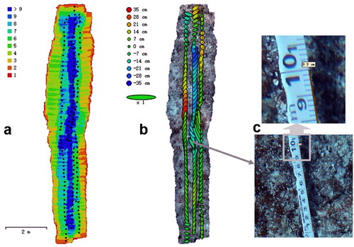
Figure 4. Statistical analysis of reference scale segments.

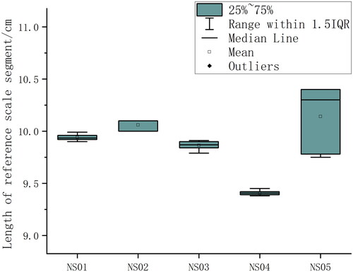
Figure 5. Analysis of coral cover from the orthomosaics. Green patches are coral colonies, red lines are the measuring tapes and blue lines are the virtual transects. The bottom three screenshots are coral recruits with different species and sizes.

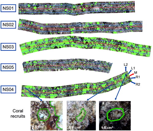
Figure 6. The estimates of percent coral cover by three methods. (a) The axes are the estimates of the three methods, which can clearly show the ranking of the estimates of the five sites. (b) The axes are the estimates of the five sites, including only the results of LIT and LITO.

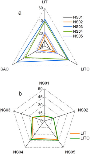
Table 3. Data quality and accuracy.

Sites		NS01	NS02	NS03	NS04	NS05
RMS reprojection error/pix		0.85	0.91	0.99	0.86	0.49
Reference scale segments	Range of values/cm	9.90–9.99	10.00–10.10	9.79–9.91	9.38–9.45	9.75–10.40
	Mean value/cm	9.94	10.06	9.86	9.41	10.14
	Sample standard deviation	0.0320	0.0516	0.0401	0.0207	0.2964
Scaling factor		0.994	1.006	0.986	0.941	1.014

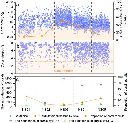
Figure 7 shows the distribution of coral size (cm²), coral cover estimates by SAO, the abundance of coral and the proportion of coral recruits at each site. To highlight the distribution of coral colonies’ size at each site, the data were transformed using the log₂, in Figure 7(a). The blue pellets represent each coral colony extracted, and the abundance of coral colonies from NS01 to NS05 is: 321, 181, 1179, 915 and 952. Figure 7(b) is a large view of the orange portion of Figure 7(a), with coral colony size (cm²) on the vertical axis. To make the distribution of coral recruits clearer, the size of the blue particles corresponds to the size of the coral colonies, and the dotted orange line is the threshold for coral recruits. The abundance of coral recruits from NS01 to NS05 is:100, 11, 7, 100 and 236, and the smallest coral recruit we identified from NS01 to NS05 is: 0.36, 0.67, 2.05, 0.59, 0.54. In Figure 7(c), the proportion of coral recruits from NS01 to NS05 is: 31.2%, 6.1%, 0.6%, 10.9%, 24.8%, respectively.

Figure 7. Comparative analysis of the LITO and SAO methods. (a) The blue pellets represent each coral colony extracted. To highlight the distribution of coral colonies’ size at each site, the data were transformed using the log₂. (b) A larger view of the orange section of Figure 7(a) makes the distribution of coral recruits clearer. (c) The abundance of corals involved in the estimate of coral cover by the LITO and SAO methods and proportions of coral recruits.

4. Discussion

The estimates of percent coral cover by LIT and LITO are similar, as shown in Figure 6(b). Though the estimates for NS02 from both methods are the same, the LIT estimates of the other four sites are slightly below the LITO estimates. It is well known that LIT surveys use the scale value of the measuring tape itself as the length of the transect to calculate the coral cover estimate and ignore the sagging, bowing and body of the measuring tape (used to tighten the tape and minimize current-induced motion). Therefore, in practice, the true length of the transect is often less than the length of the tape. However, each transect in this study is approximately 10 m in length, so the impact of these errors is minimal; though, the error increases as the length of the transect increases. In actual survey work, the length of the transect line is usually recommended to be 50 m or longer (English et al. 1997; Hill and Wilkinson 2004). However, LITO methods can reduce the influence of these tape errors by using reference scale segments to correct the length of the transect. Thus, the transect length used for calculations is closer to the real length and estimates of percent coral cover are more accurate.

The greater the number of corals involved in the coral cover estimate calculation, the more representative the estimate is of the coral distribution in the study area. SAO has a distinct advantage over LIT or LITO in terms of coral abundance, as shown in Figure 7(a,c). NS03–NS05, which have higher coral cover estimate, have greater differences in coral abundance between LITO and SAO. SAO can also be used to analyse the distribution of corals of different ages (ignoring the incomplete corals cut-off at the edge of orthomosaics during buffer analysis), especially the proportion of coral recruits. In Figure 7, it can be seen that there is no correlation between the number of coral recruits and coral cover, and even NS03, which has the highest coral cover, has the lowest number and proportion of coral recruits. However, NS01, with the lowest coral cover, has the highest proportion of coral recruits. One objective reason for this is that the higher the coral cover is, the more abundant the coral larvae are, but the less space for them to settle, while areas with less coral cover provide more settlement space for coral larvae. However, it was overlooked in SAO method that maybe some recruits were growing in those ‘black areas’ which were not recorded by the perpendicular pictures during the survey. Also, the number of coral recruits is influenced by numerous other factors, such as habitat competition with algae, topography, hydrodynamics and predation by parrotfish (Edmunds 2000).

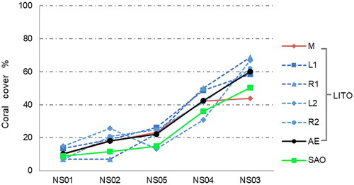
To assess the impact of random transects on coral cover estimates by LIT or LITO, we took four virtual transects on each orthomosaic, as shown by the blue lines in Figure 5. The red line (measuring tape) is denoted as M, and the blue lines are denoted as L1, L2, R1 and R2. These lines are parallel to each other, and the distance between adjacent lines is 0.25 m. Figure 8 shows estimates of percent coral cover by SAO, as well as those of the five LITO transects (M, L1, L2, R1 and R2) and their average estimates (AEs). At each site it can be seen that most LITO coral cover estimates are larger than those determined by SAO. However, there is a reversal at each site that differs from the conclusions of some scholars. For instance, Leujak and Ormond (2007) found that the LIT method overestimated principal benthic categories; Urbina-Barreto et al. (2021b) indicated that LIT generated higher coral cover estimates than did the other methods, and SAO resulted in the lowest and least variable percentages of coral cover estimates. However, there is a relatively consistent relationship between estimates by SAO and the AEs by LITO, in which the former is always smaller than the latter. Thus, AEs have greater consistency but slightly overestimate percentages relative to the estimates by SAO. The AE is a better representation than the individual LIT or LITO estimate.

Figure 8. Estimates of percent coral cover by LITO and SAO.

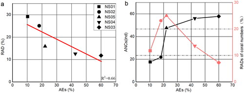
Figure 9(a) shows the AEs and the relative average deviation (RAD) of coral cover estimates by LITO (M, L1, L2, R1 and R2 transects). The RAD is negatively correlated with AE, which indicates that the estimation of coral cover by LITO or LIT is more reliable and consistent when coral cover is higher, and the probability of overestimation is lower. The average number of corals (ANC) (M, L1, L2, R1 and R2 transects) is positively correlated with AE, but the correlation is not linear, as shown in Figure 9(b). This may be related to the fact that areas with higher coral cover are more likely to have larger corals. However, the RAD of coral abundances (M, L1, L2, R1 and R2 transects) first increases and then decreases, which also indicates that areas with higher coral cover are more likely to have larger corals. A smaller RAD of coral abundances is beneficial for reliability and consistency in the estimation of coral cover by LITO or LIT. In addition, the highest coral cover in this article is only 50.4%. We will need to obtain more data (higher coral cover) to verify our conclusions.

Figure 9. (a) The relationship between AEs and RADs of coral cover estimates by LITO. (b) The relationship between AEs and ANCs and RADs of coral abundances.

Although the coral cover estimate, especially the overestimate, by the LIT method is highly random, it is still one of the common coral reef survey methods. Currently, there are few reports of underwater SfM techniques, especially in the field of coral reef ecosystem investigation and research in China. According to our conclusions, AEs can effectively reduce the unreliability and inconsistency in LIT or LITO results but can also cause some overestimation. Therefore, it is suggested that parallel transects can be appropriately added, or transects lengthened, to reduce the influence of unreliability and inconsistency when the LIT method is used for coral cover surveys.

5. Conclusion

With the continued improvement of software and hardware, as well as many successful applications in coral reef ecosystems, underwater SfM technology is likely to become the new standard for coral reef surveying (Obura et al. 2019; D'Urban Jackson et al. 2020). This method can quantify many characteristics of coral reef ecosystems, such as slope, fractal dimension, surface complexity, coral cover, colony size and abundance (Storlazzi et al. 2016; Fukunaga et al. 2019; Price et al. 2019; Carlot et al. 2020). These are important factors to consider for gaining insight into the causes and magnitude of threats to coral reefs (Palma et al. 2017) and for developing conservation strategies (Anelli et al. 2019). Attempts by governments, associations and agencies to protect coral reef ecosystems have not succeeded in stopping large-scale degradation (Palma et al. 2017), but more international efforts are underway (e.g. an ambitious effort is underway to protect 30% of Earth’s land and sea areas by 2030 as part of the recently adopted Kunming–Montreal Global Biodiversity Framework (CBD 2022); a growing number of governments and nongovernmental actors are proposing a new global treaty to combat plastic pollution (Simon et al. 2021)). So further research is needed to fully understand the importance of new technologies and approaches for coral reef surveys and assessments.

Authors’ contributions

MW, SL, XX, JY, CC and XS contributed to the study conception and design. Field work and image acquisition were performed by MW, XX, CC and XS. Material preparation and data analysis were performed by SL, XX and JY. The first draft of the manuscript was written by MW and all authors commented on previous versions of the manuscript. All authors read and approved the final manuscript.

Disclosure statement

All authors certify that they have no affiliations with or involvement in any organization or entity with any financial interest or non-financial interest in the subject matter or materials discussed in this manuscript.

Additional information

Funding

MW was supported by a Science and Technology Development Foundation of South China Sea Bureau, Ministry of Natural Resources (No. 230105).

References

- Abadie A, Boissery P, Viala C. 2018. Georeferenced underwater photogrammetry to map marine habitats and submerged artificial structures. Photogramm Rec. 33(164):448–469. doi: 10.1111/phor.12263.
- Adjeroud M, Kayal M, Iborra-Cantonnet C, Vercelloni J, Bosserelle P, Liao V, Chancerelle Y, Claudet J, Penin L. 2018. Recovery of coral assemblages despite acute and recurrent disturbances on a South Central Pacific reef. Sci Rep. 8(1):9680. doi: 10.1038/s41598-018-27891-3.
- Alvarez-Filip L, Dulvy NK, Gill JA, Côté IM, Watkinson AR. 2009. Flattening of Caribbean coral reefs: region-wide declines in architectural complexity. Proc Biol Sci. 276(1669):3019–3025. doi: 10.1098/rspb.2009.0339.
- Anelli M, Julitta T, Fallati L, Galli P, Rossini M, Colombo R. 2019. Towards new applications of underwater photogrammetry for investigating coral reef morphology and habitat complexity in the Myeik Archipelago, Myanmar. Geocarto Int. 34(5):459–472. doi: 10.1080/10106049.2017.1408703.
- Antervedi LGP, Chen Z, Anand H, Martin R, Arrowsmith R, Das J. 2021. Terrain-relative diver following with autonomous underwater vehicle for coral reef mapping. 2021 IEEE 17th International Conference on Automation Science and Engineering (CASE); Lyon, France. p. 2307–2312. doi: 10.1109/CASE49439.2021.9551624.
- Bayley D. 2019. Empirical and mechanistic approaches to understanding and projecting change in coastal marine communities [dissertation]. London: University College.
- Bayley DT, Mogg AO, Koldewey H, Purvis A. 2019. Capturing complexity: field-testing the use of ‘structure from motion’ derived virtual models to replicate standard measures of reef physical structure. PeerJ. 7:e6540. doi: 10.7717/peerj.6540.
- Bejarano S, Mumby PJ, Sotheran I. 2011. Predicting structural complexity of reefs and fish abundance using acoustic remote sensing (RoxAnn). Mar Biol. 158(3):489–504. doi: 10.1007/s00227-010-1575-5.
- Bellwood DR, Hughes TP, Folke C, Nyström M. 2004. Confronting the coral reef crisis. Nature. 429(6994):827–833. doi: 10.1038/nature02691.
- Bennecke S, Kwasnitschka T, Metaxas A, Dullo WC. 2016. In situ growth rates of deep-water octocorals determined from 3D photogrammetric reconstructions. Coral Reefs. 35(4):1227–1239. doi: 10.1007/s00338-016-1471-7.
- Birrell CL, McCook LJ, Willis BL, Diaz-Pulido GA. 2008. Effects of benthic algae on the replenishment of corals and the implications for the resilience of coral reefs. In: Oceanography and marine biology. CRC Press; p. 31–70.
- Brandl SJ, Goatley CH, Bellwood DR, Tornabene L. 2018. The hidden half: ecology and evolution of cryptobenthic fishes on coral reefs. Biol Rev Camb Philos Soc. 93(4):1846–1873. doi: 10.1111/brv.12423.
- Burns JHR, Delparte D, Gates RD, Takabayashi M. 2015. Utilizing underwater three-dimensional modeling to enhance ecological and biological studies of coral reefs. Int Arch Photogramm Remote Sens Spatial Inf Sci. XL-5/W5:61–66. doi: 10.5194/isprsarchives-XL-5-W5-61-2015.
- Bythell J, Pan P, Lee J. 2001. Three-dimensional morphometric measurements of reef corals using underwater photogrammetry techniques. Coral Reefs. 20(3):193–199. doi: 10.1007/s003380100157.
- Carlot J, Rovère A, Casella E, Harris D, Grellet-Muñoz C, Chancerelle Y, Dormy E, Hedouin L, Parravicini V. 2020. Community composition predicts photogrammetry-based structural complexity on coral reefs. Coral Reefs. 39(4):967–975. doi: 10.1007/s00338-020-01916-8.
- Casella E, Collin A, Harris D, Ferse S, Bejarano S, Parravicini V, Hench JL, Rovere A. 2017. Mapping coral reefs using consumer-grade drones and structure from motion photogrammetry techniques. Coral Reefs. 36(1):269–275. doi: 10.1007/s00338-016-1522-0.
- CBD. 2022. Kunming-Montreal global biodiversity framework. Proceedings of the Conference of Parties to the Convention on Biological Diversity Fifteenth Meeting CBD/COP/15/L.25.
- Chave KE, Smith SV, Roy KJ. 1972. Carbonate production by coral reefs. Mar Geol. 12(2):123–140. doi: 10.1016/0025-3227(72)90024-2.
- Czechowska K, Feldens P, Tuya F, Cosme de Esteban M, Espino F, Haroun R, Schönke M, Otero-Ferrer F. 2020. Testing side-scan sonar and multibeam echosounder to study black coral gardens: a case study from Macaronesia. Remote Sens. 12(19):3244. doi: 10.3390/rs12193244.
- D'Urban Jackson T, Williams GJ, Walker-Springett G, Davies AJ. 2020. Three-dimensional digital mapping of ecosystems: a new era in spatial ecology. Proc Biol Sci. 287(1920):20192383. doi: 10.1098/rspb.2019.2383.
- Edmunds PJ. 2000. Patterns in the distribution of juvenile corals and coral reef community structure in St. John, US Virgin Islands. Mar Ecol Prog Ser. 202:113–124. doi: 10.3354/meps202113.
- Elise S, Urbina-Barreto I, Pinel R, Mahamadaly V, Bureau S, Penin L, Adjeroud M, Kulbicki M, Bruggemann JH.,. 2019. Assessing key ecosystem functions through soundscapes: a new perspective from coral reefs. Ecol Indic. 107:105623. doi: 10.1016/j.ecolind.2019.105623.
- English S, Wilkinson C, Baker V. 1997. Survey manual for tropical marine resources. 2nd ed. Townsville: Australian Institute of Marine Science.
- Fallati L, Saponari L, Savini A, Marchese F, Corselli C, Galli P. 2020. Multi-temporal UAV data and object-based image analysis (OBIA) for estimation of substrate changes in a post-bleaching scenario on a Maldivian reef. Remote Sens. 12(13):2093. doi: 10.3390/rs12132093.
- Ferrari R, Bryson M, Bridge T, Hustache J, Williams SB, Byrne M, Figueira W. 2016. Quantifying the response of structural complexity and community composition to environmental change in marine communities. Glob Chang Biol. 22(5):1965–1975. doi: 10.1111/gcb.13197.
- Ferrari R, Figueira WF, Pratchett MS, Boube T, Adam A, Kobelkowsky-Vidrio T, Doo SS, Atwood TB, Byrne M. 2017. 3D photogrammetry quantifies growth and external erosion of individual coral colonies and skeletons. Sci Rep. 7(1):16737. doi: 10.1038/s41598-017-16408-z.
- Friedman A, Pizarro O, Williams SB, Johnson-Roberson M. 2012. Multi-Scale measures of rugosity, slope and aspect from benthic stereo image reconstructions. PLoS One. 7(12):e50440. doi: 10.1371/journal.pone.0050440.
- Fukunaga A, Burns JH, Craig BK, Kosaki RK. 2019. Integrating three dimensional benthic habitat characterization techniques into ecological monitoring of coral reefs. JMSE. 7(2):27. doi: 10.3390/jmse7020027.
- Gardner TA, Côté IM, Gill JA, Grant A, Watkinson AR. 2003. Long-term region-wide declines in Caribbean corals. Science. 301(5635):958–960. doi: 10.1126/science.1086050.
- Giles AB, Ren K, Davies JE, Abrego D, Kelaher B. 2023. Combining drones and deep learning to automate coral reef assessment with RGB imagery. Remote Sens. 15(9):2238. doi: 10.3390/rs15092238.
- Goodman JA, Lay M, Ramirez L, Ustin SL, Haverkamp PJ. 2020. Confidence levels, sensitivity, and the role of bathymetry in coral reef remote sensing. Remote Sens. 12(3):496. doi: 10.3390/rs12030496.
- Gove JM, Williams GJ, Lecky J, Brown E, Conklin E, Counsell C, Davis G, Donovan MK, Falinski K, Kramer L, et al. 2023. Coral reefs benefit from reduced land–sea impacts under ocean warming. Nature. 621(7979):536–542. doi: 10.1038/s41586-023-06394-w.
- Hearn CJ. 2011. Perspectives in coral reef hydrodynamics. Coral Reefs. 30(S1):1–9. doi: 10.1007/s00338-011-0752-4.
- Hedley J, Roelfsema C, Chollett I, Harborne A, Heron S, Weeks S, Skirving W, Strong A, Eakin C, Christensen T, et al. 2016. Remote sensing of coral reefs for monitoring and management: a review. Remote Sens. 8(2):118. doi: 10.3390/rs8020118.
- Hedley JD, Roelfsema CM, Phinn SR, Mumby PJ. 2012. Environmental and sensor limitations in optical remote sensing of coral reefs: implications for monitoring and sensor design. Remote Sens. 4(1):271–302. doi: 10.3390/rs4010271.
- Heron SF, Maynard JA, Van Hooidonk R, Eakin CM. 2016. Warming trends and bleaching stress of the world’s coral reefs 1985–2012. Sci Rep. 6(1):38402. doi: 10.1038/srep38402.
- Hill J, Wilkinson CLIVE. 2004. Methods for ecological monitoring of coral reefs. Townsville: Australian Institute of Marine Science. doi: 10.1017/CBO9781107415324.004.
- Hochberg EJ, Atkinson MJ, Andréfouët S. 2003. Spectral reflectance of coral reef bottom-types worldwide and implications for coral reef remote sensing. Remote Sens Environ. 85(2):159–173. doi: 10.1016/S0034-4257(02)00201-8.
- Hoegh-Guldberg O, Mumby PJ, Hooten AJ, Steneck RS, Greenfield P, Gomez E, Harvell CD, Sale PF, Edwards AJ, Caldeira K, et al. 2007. Coral reefs under rapid climate change and ocean acidification. Science. 318(5857):1737–1742. doi: 10.1126/science.115250.
- Hughes TP, Kerry JT, Álvarez-Noriega M, Álvarez-Romero JG, Anderson KD, Baird AH, Babcock RC, Beger M, Bellwood DR, Berkelmans R, et al. 2017. Global warming and recurrent mass bleaching of corals. Nature. 543(7645):373–377. doi: 10.1038/nature21707.
- Joyce KE, Phinn SR. 2013. Spectral index development for mapping live coral cover. J Appl Remote Sens. 7(1):073590. doi: 10.1117/1.JRS.7.073590.
- Joyce KE, Phinn SR, Roelfsema CM. 2013. Live coral cover index testing and application with hyperspectral airborne image data. Remote Sens. 5(11):6116–6137. doi: 10.3390/rs5116116.
- Knudby A, LeDrew E, Newman C. 2007. Progress in the use of remote sensing for coral reef biodiversity studies. Prog Phys Geogr. 31(4):421–434. doi: 10.1177/0309133307081292.
- Lamb JB, Willis BL, Fiorenza EA, Couch CS, Howard R, Rader DN, True JD, Kelly LA, Ahmad A, Jompa J, et al. 2018. Plastic waste associated with disease on coral reefs. Science. 359(6374):460–462. doi: 10.1126/science.aar332.
- Lange ID, Perry CT. 2020. A quick, easy and non-invasive method to quantify coral growth rates using photogrammetry and 3D model comparisons. Methods Ecol Evol. 11(6):714–726. doi: 10.1111/2041-210X.13388.
- Lavy A, Eyal G, Neal B, Keren R, Loya Y, Ilan M. 2015. A quick, easy and non-intrusive method for underwater volume and surface area evaluation of benthic organisms by 3D computer modelling. Methods Ecol Evol. 6(5):521–531. doi: 10.1111/2041-210X.12331.
- Le Quilleuc A, Collin A, Jasinski MF, Devillers R. 2021. Very high-resolution satellite-derived bathymetry and habitat mapping using Pleiades-1 and ICESat-2. Remote Sens. 14(1):133. doi: 10.3390/rs14010133.
- Lechene MAA, Haberstroh AJ, Byrne M, Figueira W, Ferrari R. 2019. Optimising sampling strategies in coral reefs using large-areas mosaics. Remote Sens. 11(24):2907. doi: 10.3390/rs11242907.
- Leon JX, Roelfsema CM, Saunders MI, Phinn SR. 2015. Measuring coral reef terrain roughness using ‘Structure-from-Motion’ close-range photogrammetry. Geomorphology. 242:21–28. doi: 10.1016/j.geomorph.2015.01.030.
- Leujak W, Ormond RFG. 2007. Comparative accuracy and efficiency of six coral community survey methods. J Exp Mar Biol Ecol. 351(1–2):168–187. doi: 10.1016/j.jembe.2007.06.028.
- Liao ZH. 2021. Spatial distribution of coral community and benthic algae and their ecological impacts across the south china sea [dissertation]. Guangxi University.
- McCarthy J, Benjamin J. 2014. Multi-image photogrammetry for underwater archaeological site recording: an accessible, diver-based approach. J Mari Arch. 9(1):95–114. doi: 10.1007/s11457-014-9127-7.
- Modasshir M, Rekleitis I. 2020. Enhancing coral reef monitoring utilizing a deep semi-supervised learning approach. 2020 IEEE International Conference on Robotics and Automation (ICRA). p. 1874–1880. doi: 10.1109/ICRA40945.2020.9196528.
- Montalbetti E, Fallati L, Casartelli M, Maggioni D, Montano S, Galli P, Seveso D. 2022. Reef complexity influences distribution and habitat choice of the corallivorous seastar Culcita schmideliana in the Maldives. Coral Reefs. 41(2):253–264. doi: 10.1007/s00338-022-02230-1.
- Muhamad MAH, Hasan RC, Said NM, Said MSM, Razali R. 2023. Marine habitat mapping using multibeam echosounder survey and underwater video observations: a case study from Tioman marine park. IOP Conf Ser: Earth Environ Sci. 1240(1):012006. doi: 10.1088/1755-1315/1240/1/012006.
- Neyer F, Nocerino E, Gruen A. 2018. Monitoring coral growth– the dichotomy between underwater photogrammetry and geodetic control network. Int Arch Photogramm Remote Sens Spatial Inf Sci. XLII-2:759–766. doi: 10.5194/isprs-archives-XLII-2-759-2018.
- Nocerino E, Menna F, Gruen A, Troyer M, Capra A, Castagnetti C, Rossi P, Brooks AJ, Schmitt RJ, Holbrook SJ. 2020. Coral reef monitoring by scuba divers using underwater photogrammetry and geodetic surveying. Remote Sens. 12(18):3036. doi: 10.3390/rs12183036.
- Obura DO, Aeby G, Amornthammarong N, Appeltans W, Bax N, Bishop J, Brainard RE, Chan S, Fletcher P, Gordon TAC, et al. 2019. Coral reef monitoring, reef assessment technologies, and ecosystem-based management. Front Mar Sci. 6:580. doi: 10.3389/fmars.2019.00580.
- Palma M, Rivas Casado M, Pantaleo U, Cerrano C. 2017. High resolution orthomosaics of African coral reefs: a tool for wide-scale benthic monitoring. Remote Sens. 9(7):705. doi: 10.3390/rs9070705.
- Penin L, Michonneau F, Baird AH, Connolly SR, Pratchett MS, Kayal M, Adjeroud M. 2010. Early post-settlement mortality and the structure of coral assemblages. Mar Ecol Prog Ser. 408:55–64. doi: 10.3354/meps08554.
- Perry CT, Alvarez-Filip L, Graham NAJ, Mumby PJ, Wilson SK, Kench PS, Manzello DP, Morgan KM, Slangen ABA, Thomson DP, et al. 2018. Loss of coral reef growth capacity to track future increases in sea level. Nature. 558(7710):396–400. doi: 10.1038/s41586-018-0194-z.
- Pinheiro HT, MacDonald C, Santos RG, Ali R, Bobat A, Cresswell BJ, Francini-Filho R, Freitas R, Galbraith GF, Musembi P, et al. 2023. Plastic pollution on the world’s coral reefs. Nature. 619(7969):311–316. doi: 10.1038/s41586-023-06113-5.
- Price DM, Robert K, Callaway A, Lo Lacono C, Hall RA, Huvenne VA. 2019. Using 3D photogrammetry from ROV video to quantify cold-water coral reef structural complexity and investigate its influence on biodiversity and community assemblage. Coral Reefs. 38(5):1007–1021. doi: 10.1007/s00338-019-01827-3.
- Rossi P, Castagnetti C, Capra A, Brooks AJ, Mancini F. 2020. Detecting change in coral reef 3D structure using underwater photogrammetry: critical issues and performance metrics. Appl Geomat. 12(S1):3–17. doi: 10.1007/s12518-019-00263-w.
- Santos RG, Machovsky-Capuska GE, Andrades R. 2021. Plastic ingestion as an evolutionary trap: toward a holistic understanding. Science. 373(6550):56–60. doi: 10.1126/science.abh0945.
- Simon N, Raubenheimer K, Urho N, Unger S, Azoulay D, Farrelly T, Sousa J, van Asselt H, Carlini G, Sekomo C, et al. 2021. A binding global agreement to address the life cycle of plastics. Science. 373(6550):43–47. doi: 10.1126/science.abi90.
- Stella JS, Pratchett MS, Hutchings P, Jones GP. 2011. Coralasscociated invertebrates: diversity, ecological importance and vulnerability to disturbance. Oceanogr Mar Biol. 49:43–104.
- Storlazzi CD, Dartnell P, Hatcher GA, Gibbs AE. 2016. End of the chain? Rugosity and fine-scale bathymetry from existing underwater digital imagery using structure-from-motion (SfM) technology. Coral Reefs. 35(3):889–894. 8-016-1462-8 doi: 10.1007/s0033.
- Urbina-Barreto I, Chiroleu F, Pinel R, Fréchon L, Mahamadaly V, Elise S, Kulbicki M, Quod J-P, Dutrieux E, Garnier R, et al. 2021a. Quantifying the shelter capacity of coral reefs using photogrammetric 3D modelling, from colonies to reefscapes. Ecol Indicat. 121:107151. doi: 10.1016/j.ecolind.2020.107151.
- Urbina-Barreto I, Garnier R, Elise S, Pinel R, Dumas P, Mahamadaly V, Facon M, Bureau S, Peignon C, Quod J-P, et al. 2021b. Which method for which purpose? A comparison of line intercept transect and underwater photogrammetry methods for coral reef surveys. Front Mar Sci. 8:636902. doi: 10.3389/fmars.2021.636902.
- Westoby MJ, Brasington J, Glasser NF, Hambrey MJ, Reynolds JM. 2012. ‘Structure-from-Motion’ photogrammetry: a low-cost, effective tool for geoscience applications. Geomorphology. 179:300–314. doi: 10.1016/j.geomorph.2012.08.021.
- Young GC, Dey S, Rogers AD, Exton D. 2017. Cost and time-effective method for multi-scale measures of rugosity, fractal dimension, and vector dispersion from coral reef 3D models. PLoS One. 12(4):e0175341. doi: 10.1371/journal.pone.0175341.
- Zawada KJ, Madin JS, Baird AH, Bridge TC, Dornelas M. 2019. Morphological traits can track coral reef responses to the Anthropocene. Funct Ecol. 33(6):962–975. doi: 10.1111/1365-2435.
- Zhou J, Zhou N, Che Y, Gao J, Zhao L, Huang H, Chen Y. 2022. Design and development of an autonomous underwater helicopter for ecological observation of coral reefs. Sensors (Basel). 22(5):1770. doi: 10.3390/s22051770.