The shape of low-concentration dose–response functions for benzene: implications for human health risk assessment

Abstract

Are dose–response relationships for benzene and health effects such as myelodysplastic syndrome (MDS) and acute myeloid leukemia (AML) supra-linear, with disproportionately high risks at low concentrations, e.g. below 1 ppm? To investigate this hypothesis, we apply recent mode of action (MoA) and mechanistic information and modern data science techniques to quantify air benzene-urinary metabolite relationships in a previously studied data set for Tianjin, China factory workers. We find that physiologically based pharmacokinetics (PBPK) models and data for Tianjin workers show approximately linear production of benzene metabolites for air benzene (AB) concentrations below about 15 ppm, with modest sublinearity at low concentrations (e.g. below 5 ppm). Analysis of the Tianjin worker data using partial dependence plots reveals that production of metabolites increases disproportionately with increases in air benzene (AB) concentrations above 10 ppm, exhibiting steep sublinearity (J shape) before becoming saturated. As a consequence, estimated cumulative exposure is not an adequate basis for predicting risk. Risk assessments must consider the variability of exposure concentrations around estimated exposure concentrations to avoid over-estimating risks at low concentrations. The same average concentration for a specified duration is disproportionately risky if it has higher variance. Conversely, if chronic inflammation via activation of inflammasomes is a critical event for induction of MDS and other health effects, then sufficiently low concentrations of benzene are predicted not to cause increased risks of inflammasome-mediated diseases, no matter how long the duration of exposure. Thus, we find no evidence that the dose–response relationship is supra-linear at low doses; instead sublinear or zero excess risk at low concentrations is more consistent with the data. A combination of physiologically based pharmacokinetic (PBPK) modeling, Bayesian network (BN) analysis and inference, and partial dependence plots appears a promising and practical approach for applying current data science methods to advance benzene risk assessment.

Keywords:

• Benzene metabolism
• supralinearity
• PBPK model
• machine learning
• Bayesian networks
• Chinese workers

Introduction: are low-concentration benzene dose–response functions supralinear?

Supralinear dose–response functions – that is, dose–response functions in which low doses are disproportionately potent in causing harm – have sometimes been proposed as describing the risks from many well-studied public and occupational hazards. Examples include asbestos, benzene, lead, particulate air pollution, and ionizing radiation. A suggested risk management implication is that exposure concentrations must be driven to zero, or close to it, to adequately protect human health (Hornung and Lanphear 2014; Lanphear 2017). Some of these concerns have been challenged as statistically flawed or as biologically unrealistic (Waddell 2006; Hornung and Lanphear 2014). For example, studies that identify supralinear dose–response relationships can be questioned if they fail to control fully for important potential confounders, such as misclassified smoking (Hamling et al. 2019). Omitted and residual confounding by smoking can create significant associations between some common exposure metrics (e.g. blood lead levels) and adverse health effects (e.g. cardiovascular mortality and morbidity) whether or not the former affect the latter. Misattributing risk caused by a confounder to exposure creates the appearance of a supra-linear dose–response function since risk fails to decline as exposure decreases, in effect spreading the same risk over fewer units of exposure.

For many other agents, including asbestos, mineral dusts and particulate matter, and ionizing radiation, it has recently been discovered that major exposure-associated adverse health effects are mediated by chronic inflammation and activation of a specific signaling complex (the NLRP3 inflammasome) with an activation threshold, such that low exposure concentrations do not trigger inflammasome assembly and activation and resulting increases in disease risks (Bogen 2019; Cox 2019; Du et al. 2019; Wei et al. 2019). For other chemicals, causal mechanisms of adverse outcomes and modes of action are less clear. For these chemicals, careful review is needed to assess the biological plausibility of supralinear dose–response function for low exposure concentrations. The purpose of this paper is to provide such an assessment for benzene, focusing specifically on whether production of putative harmful metabolites of benzene is supralinear at low concentrations.

The suggestion that low-dose metabolism of benzene is supralinear has been advanced using data from factory workers in Tianjin, China (Rappaport et al. 2009, 2010). Applying nonlinear parametric regression models that take a ratio Y/X as the dependent variable and X as the independent variable, where Y = measured quantity of a benzene metabolite and X = estimated concentration of benzene in inhaled air to data for factory workers in Tianjin revealed that the ratio Y/X increases as X decreases, for various metabolites Y (Rappaport et al. 2010). This observation was interpreted as strong evidence for a supralinear dose–response explained by an unknown enzyme that becomes saturated at concentrations below the detection limit for benzene, in preference to an alternative explanation that the apparent supralinearity reflects unrealistic assumptions about unmeasured background levels of benzene exposure (since the supralinearity finding disappears if “background” concentrations are defined as those for workers without occupational exposures) (Rappaport et al. 2013). More recent work applying nonparametric statistical and machine learning techniques to the Tianjin data to avoid potential biases from parametric regression modeling found no departures from linear metabolism at low exposure concentrations, but clarified that a ratio Y/X can increase as X approaches zero even if metabolism is linear, if estimated values are measured with error variance, as in the Tianjin data (McNally et al. 2017; Cox et al. 2017). In effect, the probability of having estimated X value near zero and estimated Y values well above 0 is sufficient to make their ratio increase as the estimated X value approaches zero, even if the ratio of their true values remains constant.

To further advance understanding of the shapes of benzene metabolism and dose–response relationships at low exposure concentrations in air, the following sections address the following five related research questions:

1. Which metabolites and markers best predict human health risks from low levels of benzene exposure (and why)?

2. How do levels of metabolites and markers change with levels of benzene in inhaled air, and with levels of other factors (e.g. diet, alcohol consumption, cigarette smoking)?

3. How much do inter-individual heterogeneity and variability affect benzene metabolism?

4. How much intra-individual variability is there in benzene metabolism?

5. At what levels do different metabolites and relevant markers predict increased risk of adverse health effects from benzene exposure?

Questions 1 and 5 are addressed based on existing literature. To obtain new insights into questions 2–4, we also apply current data science techniques to identify and quantify potential causal relationships between inhaled benzene and levels of relevant benzene metabolites in the Tianjin factory worker data.

Benzene markers and metabolites relevant for human health

Benzene metabolism and pharmacokinetics

Human metabolism of benzene has been intensively studied and elucidated. Figure 1(a,b) shows major benzene metabolic pathways, both as sequences of molecular structures (Figure 1(a)) and as a pathway schematic (Figure 1(b)) with metabolites (blue) and metabolizing enzymes (black); these can be explored via the interactive WikiPathway (Slenter et al. 2018) from which Figure 1(b) is taken. Physiologically based pharmacokinetic (PBPK) models have been developed and validated for benzene metabolism in humans, mice, rats, and other species (Knutsen et al. 2013). Metabolism and distribution of benzene in liver, bone marrow, and other tissue groups have been compared across species and their interindividual and intraindividual variability in human populations have been studied and modeled quantitatively in population PBPK models (Yokley et al. 2006). In discussing benzene metabolism, different authors focus on trans, trans-muconaldehyde (ttM), E,E-muconaldehyde, or trans, trans-muconic acid (t,t-MA or simply MA) (i.e. the diene dialdehyde and its dicarboxylic acid metabolite, respectively) as indicators of open-ring products formed by cytochrome P4502E1 (CYP) metabolism. We follow this mixed usage in summarizing relevant results from the literature.

Figure 1. (a) Chemical structures of human metabolites of benzene. Source: Rappaport et al. (2010). (b) Pathway schematic showing major metabolites (blue) and metabolizing enzymes (black) [muconic acid (MA) not shown]. Right side: side pathway schematic is from: https://www.wikipathways.org/index.php/Pathway:WP3891#nogo2.

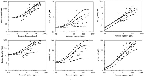
Figure 2 shows the compartmental structure of a recent benzene PBPK model for humans (Knutsen et al. 2013). Figure 3 compares model predictions to observations of metabolites in data not used in building the model. (The scales in Figure 3 are logarithmic, so predictions and data are compared across estimated exposure concentrations that differ by several orders of magnitude.) Estimated rates of human conversion of benzene to muconic acid (MA) and phenylmercapturic acid (PMA), phenol (PH), catechol (CA), hydroquinone (HQ), and benzenetriol (BT) in the model were validated using urinary benzene metabolite data from Chinese benzene workers. Although there is substantial interindividual variability, as reflected in the large vertical scatter in Figure 3, the PBPK model predictions pass through the observed data clouds, and in this sense roughly describe the data. Other PBPK models for benzene have been developed over the past 30 years and at least partially validated by comparing their predictions to observations in data sets not used in developing them, although most do not show bone marrow as a separate compartment. Similar to Figure 3, these PBPK models predict linear or sublinear (upward-curving, as detoxifying pathways begin to saturate) production of metabolites as a function of air benzene concentrations, for air benzene concentrations below about 10 ppm. We defer to the references for details of these PBPK models, but note that the approximate linearity of metabolite production as exposure concentration approaches zero is a property of a broad class of classical (compartmental) pharmacokinetic and PBPK models at low doses (Cox 1995). Saturation of metabolite production begins at air benzene concentrations between about 10 ppm and about 100 ppm.

Figure 2. Compartmental structure of a recent PBPK model for human metabolism of benzene. (Source: Knutsen et al. 2013).

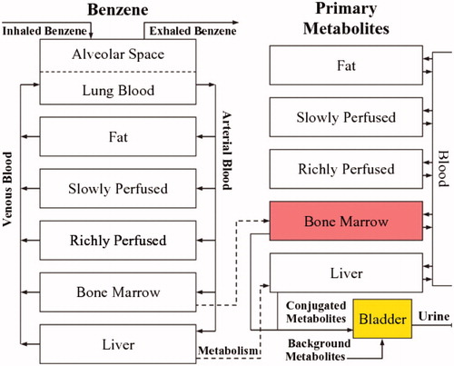
Figure 3. Comparison of benzene PBPK model predictions (solid lines) and uncertainty bands (dashed lines, representing ±2 standard deviations) to data (points) not used in building the model. MA: muconic acid; PMA: phenylmercapturic acid; PH: phenol; CAT: catechol; HQ: hydroquinone; BT: benzenetriol. (Source: Knutsen et al. 2013).

Benzene health effects and hypothesized causal biological mechanisms

Major health effects of concern for benzene-exposed workers are acute myeloid leukemia (AML) and myelodysplastic syndrome (MDS), although high concentrations (especially > 100 ppm) can also damage bone marrow and kill hematopoietic progenitor cells, causing bone marrow failure and aplastic anemia (Smith 1996; Das et al. 2012; Schnatter et al. 2012; Rushton et al. 2014). Some epidemiological data sets and statistical models have also identified associations between benzene exposure and other illnesses, especially non-Hodgkin’s lymphomas, although the evidence is mixed and causality is uncertain (Galbraith et al. 2010; Teras et al. 2019).

A central challenge for dose–response modeling of benzene health effects at relatively low concentrations of air benzene is that the specific metabolites and biological mechanisms involved in causing MDS and AML and other effects have not yet been definitively identified, although several theories and supporting evidence have been advanced (Arnold et al. 2013). Some papers interpret the fact that benzene and its reactive metabolites react with a variety of proteins and DNA in a variety of test systems as mechanistic evidence that occupational levels of benzene cause AML. For example, Grigoryan et al. (2018) state that “The fact that these diverse human serum albumin modifications differed between benzene-exposed and control workers suggests that benzene can increase leukemia risks via multiple pathways involving a constellation of reactive molecules.” However, most of the changes discussed (e.g. formation of albumin adducts in blood serum in this example, or induction of micronuclei in peripheral blood lymphocytes in other papers) have no clear causal relevance for health risks, as they are not validated markers for increased risk of MDS, AML or other adverse health effects caused by benzene (Hack et al. 2010). We focus on health-relevant markers, i.e. observable changes that act through identified causal pathways or modes of action to increase MDS and AML risks.

Most current research accepts that benzene acts by forming myelotoxic metabolites that concentrate in the bone marrow, where they damage early hematopoietic stem cells (HSCs), myeloid progenitor cells, and the stromal microenvironment, increasing the rate of cell death and replacement. However, there are diverse theories about how these events increase risk of MDS and AML. Among them are the following.

• Two-stage clonal expansion (TSCE) mode of action for benzene carcinogenesis. A proposed traditional mode of action (MoA) for benzene-induced AML begins with enzyme-dependent metabolism, mainly via cytochrome P450-2E1 (Figure 1). The resulting toxic metabolites might interact with HSCs or other target cells in the bone marrow to create mutated (“initiated”) target cells; alternatively, it might increase the clonal proliferation (i.e. expansion) rate of such initiated cells (“promotion”). Proliferation of initiated cells (perhaps stimulated by cell death due to poisoning by toxic benzene metabolites) then increases the risk of transformation of at least one of them to AML (“progression”) (Meek and Klaunig 2010). This MoA is consistent with the general two-stage clonal expansion (TSCE) models of carcinogenesis. Richardson (2009) reports that a TSCE model in which benzene increases clonal expansion fits exposure–response data for leukemia in rubber hydrochloride production workers well, with little evidence that it increases initiation; thus, quantitative TSCE modeling suggests that benzene acts as a promoter, increasing the risk of AML by increasing the rate of proliferation of initiated cells (Richardson 2009). Such promotion is typically a threshold phenomenon (Neumann 2009).

• HSC damage, genomic instability, and reduced immune surveillance. Alternatively, it has been proposed that key events in development of benzene-induced leukemia include exposure-related increases in intracellular oxidative stress in HSCs or hematopoietic progenitor cells, dysregulation of the aryl hydrocarbon receptor (AhR), and reduced immune surveillance of HSCs in the bone marrow (Hirabayashi and Inoue 2010; McHale et al. 2012; Snyder 2012; Wang et al. 2012; Kerzic and Irons 2017). McHale et al. (2012) further postulate that benzene metabolites interact with critical genes and pathways in the HSC, leading to genotoxic, chromosomal or epigenetic abnormalities and genomic instability; stromal cell dysregulation; increased rate of death (via apoptosis) of affected HSCs and stromal cells; and proliferation of altered HSCs with unrepaired damage and chromosomal aberrations, culminating in creation of leukemic stem cells and subsequent leukemia. Others have proposed that benzene metabolites (especially 1,4-benzoquinone, i.e. p-benzoquinone) cause MDS and AML by increasing chromosomal instability and unrepaired DNA damage and AML-causing chromosomal rearrangements in HSCs (e.g. via interference with topoisomerase-mediated DNA ligation and nicking) (Son et al. 2016). However, Kerzic and Irons (2017) note that such hypotheses, which predict that cytogenetic damage in benzene-induced leukemogenesis should be similar to that in chemotherapy-induced leukemogenesis, are not consistent with cytogenetic data from benzene-exposed workers with hematopoietic diseases showing that benzene-induced AML is much more similar to de novo AML than to therapy-related AML.

• Chronic inflammation MoA. In Chinese worker data, chronic inflammation followed by an immune-mediated inflammatory response, rather than cytogenetic abnormalities per se, appears to drive initiation and progression of benzene-induced MDS and AML (Gross and Paustenbach 2018). This may help to explain earlier observations that rheumatoid arthritis and other autoimmune conditions (Anderson et al. 2009), as well as respiratory infections and other common infections (Titmarsh et al. 2014), are significantly associated with increased MDS and AML risk. The inflammatory MoA is also consistent with often-noted associations between increased reactive oxygen species (ROS) and oxidative stress in affected cells and increased risk of MDS and AML. It has recently been discovered that inflammation mediated by a specific intracellular signaling platform (the NLRP3 inflammasome) that self-assembles in the cytosol of immune cells in response to exposures above an activation threshold (Cox 2019) drives the pathogenesis of MDS (Sallman and List 2019). Recent findings that benzene induces inflammatory programmed cell death (pyroptosis) (Sallman et al. 2016; Guo et al. 2019) and autophagy (Qian et al. 2019) underscore the importance of inflammatory responses in benzene-induced pathogenesis. Although inflammation increases ROS and oxidative stress and cell turnover, thus potentially increasing formation and proliferation of HSCs with unrepaired cytogenetic damage and chromosomal aberrations, the inflammatory MoA suggests that it is the underlying inflammation that drives health risks.

The TSCE and the inflammatory MoAs raise the possibility of exposure concentration thresholds below which inhaled benzene does not increase disease risks. Promotion is typically a threshold phenomenon (Neumann 2009), e.g. because concentrations must be high enough to cause toxic damage and resulting compensating proliferation of damaged HSCs. Inflammatory responses have activation thresholds or threshold-like steep nonlinearities (e.g. ultrasensitive switches) in their dose–response functions, so that tissues are not continually being inflamed by low-level exposures; the mechanisms of these activation thresholds have been substantially elucidated (Cox 2019). (Inflammation might also play a role in clonal expansion of damaged stem cells due to continuing hyperplasia acting as a co-initiator of carcinogenesis, but this also implies a threshold (or threshold-like nonlinearity) in the dose–response function (Bogen 2019).) Thus, MoA theories for benzene-induced MDS and AML in which benzene metabolites cause chronic inflammation and resulting proliferation of damaged HSCs suggest highly sub-linear (threshold or threshold-like) dose–response functions, rather than supra-linear ones. If this is correct, then benzene exposures increase risks of MDS and AML only if concentrations and durations of exposure raise concentrations of toxic metabolites in bone marrow microenvironments sufficiently high and/or long to activate inflammasomes and cause pyroptosis and other inflammatory responses. This shifts attention back to PBPK considerations.

Relevance and use of biomarkers in predicting health effects and benzene exposures: BN models

Biomarkers are potentially useful for estimating unobserved benzene exposures (or improving estimates of concentrations measured with error) and for predicting health risks caused by exposures. The predictive value of a biomarker depends on how well it can be measured and on by how much conditioning on its measured value reduces uncertainty (e.g. the average entropy of the conditional probability distribution) of the dependent variable being predicted. For example, Figure 4 shows the structure of a Bayesian network (BN) model for quantifying conditional probabilities of some variables (e.g. various metabolites, markers and AML (the Leukemia node at the lower right)), given observed or assumed values of others. The conditional probability distribution of each variable (node in the network) depends on the values of the variables that point into it. This BN, from Hack et al. (2010), was constructed manually based on a detailed literature review of candidate markers and outcomes and verifiable, usefully accurate predictive relationships among them, given limitations in measurement techniques.

Figure 4. Proposed Bayesian network (BN) model structure. (Source: Hack et al. 2010). 8-OHdG: 8-hydroxyguanosine (a biomarker of oxidative stress); CFU-GEMM: colony-forming unit-granulocyte, erythrocyte, monocyte, megakaryocyte (a precursor to RBCs and WBCs); BFU-E: burst-forming unit-erythroid (a RBC precursor cell type); CFU-GM: colony forming unit – granulocyte-macrophage (a WBC precursor); RBC: red blood cell count; ttMA: trans, trans muconic acid; WBC: white blood cell count.

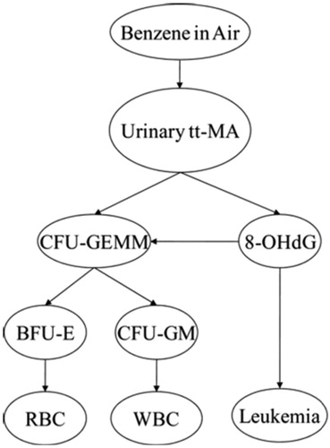
Other potentially causally relevant variables (e.g. p-benzoquinone, NLRP3 inflammasome activation, age of patient, co-exposures and co-morbidities, and so forth) are “marginalized out” of the BN model in Figure 4, meaning that they can still implicitly affect the probability of leukemia, but are not explicitly shown or conditioned on. Other investigators (or automated machine-learning programs for learning BNs directly from data) might select different markers and develop other BN models and perhaps get narrower uncertainty bands. For example, previous studies have identified urinary concentrations of SPMA (S-phenylmercapturic acid) and benzene itself as reliable indicators of recent benzene exposures, even at relatively low concentrations (e.g. 0.1 ppm for SPMA), whereas urinary tt-MA, used in Figure 4, has inadequate specificity for benzene exposures below about 1 ppm when dietary sources of sorbic acid are also present (Qu et al. 2003; Fustinoni et al. 2011; Campagna et al. 2012; Arnold et al. 2013). It might therefore be advantageous to develop a BN with SPMA and urinary benzene (UB) included as variables that can be used (i.e. conditioned on) to help predict the conditional probability distributions for other variables.

Unlike benzene PBPK modeling, which has been developed, tested and refined for decades, benzene BN modeling of benzene dose–response relationships is relatively new. Future benzene BN models may well improve on the seminal work of Hack et al. summarized in Figure 4, both by including more (and perhaps different) variables and by distinguishing between estimated and true values of benzene concentrations (and other variables measured with substantial error). The most predictively useful combinations of measurements for predicting MDS as well as AML and air benzene exposure levels have yet to be identified for such multi-variable BN models. Additional markers of chronic inflammation may be needed to complement the information already captured by the BN in Figure 4 (e.g. 8-OHdG). However, despite these limitations compared to possible future BN models, J-shaped dose–response curves for the BN model, shown in Hack et al. (2010), make clear that the BN model does not suggest supralinearity. Rather, the estimated conditional probability of AML as a function of cumulative dose is consistent with a threshold or very sublinear (J-shaped) dose–response function.

Dependence of metabolites and markers on inhaled air benzene (AB) and other factors

Simple (univariate) regression models

A well-developed literature documents increases in various markers of benzene exposure and activity with increasing air benzene (AB) concentrations, even at low doses. For example:

• Urinary benzene (UB) levels have been observed to be linearly related to work shift AB concentrations over a wide range of exposures, down to <0.2 ppm, providing a useful biomarker of benzene exposure over approximately the previous day (Weisel 2010).

• Urinary S-phenylmercapturic acid (SPMA) levels increase approximately linearly with AB concentrations between 0 and 80 ppm (Lin et al. 2008, Figure 2; see also Knutsen et al. 2013).

• tt-MA is a less specific marker for low-level benzene exposure. The problem of dietary sources for tt-MA at low exposure concentrations has already been mentioned.

• S-phenylcysteine (SPC) in albumin in human workers increased linearly with average occupational benzene exposures ranging from 0 to 23 ppm (for 8 h/d, 5 d/wk) (Bechtold and Henderson 1993).

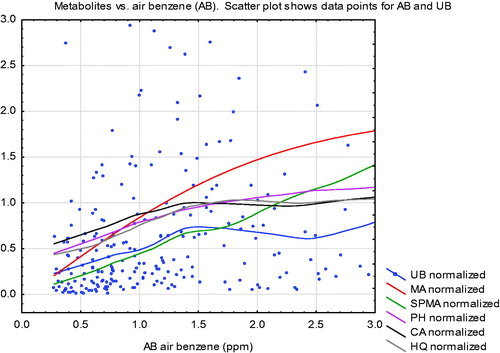
Turning from literature review to data analysis, Figure 5 shows how average urinary metabolite quantities (curves) increase with air benzene (AB) concentrations among Tianjin, China factory workers (Rappaport et al. 2010; Price et al. 2012; Cox et al. 2017). Figure 5 shows non-parametric (lowess smoothing) regression curves fit to scatter plots of urinary metabolite levels (normalized by dividing by their mean values, so that 1 on the vertical axis represents the mean value, for each metabolite) against AB concentrations from 1 to 3 ppm on the horizontal axis. (The data points shown are for UB vs. AB for workers with exposure concentrations in this range, with the vertical axis truncated at 3 to avoid scale compression due to outliers.) All curves are approximately linear for AB concentrations below 1 ppm.

Figure 5. Uriinary metabolite levels vs. air benzene (AB) at AB concentrations below 3 ppm. (Metabolites are scaled so that 1 = mean value of each metabolite in the worker population.) Curves are non-parametric (smoothing) regression curves. Data points are for urinary benzene (UB). UB: urinary benzene; MA: E, E muconic acid; SPMA: S-phenylmercapturic acid; PH: urinary phenol; CA: urinary catechol; HQ: urinary hydroquinone. Data are from Price et al. (2012).

Exploratory multivariate modeling: correlations

Univariate regression curves, with AB as the sole explanatory variable, do not explicitly account for the effects of other variables, such as age, sex, or co-exposures to toluene, in quantifying how metabolite amounts vary with AB. To better understand the interrelationships among variables, we apply the Causal Analytics Toolkit (CAT) software and methods described in Cox et al. (2017) to the Tianjin data for 177 workers with AB exposure concentrations of no more than 5 ppm and without missing data on AB or metabolites. Figure 6 shows traditional linear (Pearson’s product-moment) correlations between pairs of variables, along with frequency histograms (main diagonal) and scatter plots. These are not ideal for binary variables or for highly nonlinear relationships, but allow for quick visual exploration of the association between pairs of variables. Interpretively, the histograms on the diagonal in Figure 6 show that air benzene (AB) and its urinary metabolites are right-skewed, with long right tails indicating that a small fraction of metabolite measurements are much higher than the rest. Other entries in the table refer to pairs of variables: for each cell in the table, the variables identified on the diagonal for the row and column that intersect at the cell identify the relevant pair of variables. There are clear positive correlations in the scatterplots for some pairs of variables, such as between MA (top row and left-most column) and both UB and SPMA (bottom two rows, right-most two columns), with correlations between MA and SPMA of 0.61 and between MA and UB of 0.43 (shown in the upper right). (For ease of reference, the abbreviations of urinary metabolites of benzene are listed in the caption of Figure 5.) Likewise, Figure 7 visualizes the linear correlations in Figure 6 as a corrgram (heat map diagram at the upper left) and as a network (lower left) with stronger correlations indicated by closer distances and thicker arcs (green = positive correlation, red = negative) between variables. The upper right panel of Figure 7 provides analogous information for partial linear correlations, in which the association between each pair of variables is adjusted for levels of other variables via multiple linear regression; and the lower right presents network visualization when polychloric correlations are used instead of linear correlations for the binary variables (factory, sex, and smoking). (Only data from the 2 factories with occupational benzene exposures are included.) Again, correlations are not ideal measures for binary variables, but provide for a quick exploration.

Figure 6. Frequency histograms (main diagonal), scatter plots with kernel smoothing regression curves (below diagonal) and linear (Pearson’s product moment) correlations and significance asterisks (above diagonal) (*0.05, **0.01, ***0.001). AT: air toluene; UT: urinary toluene; Creat: creatinine.

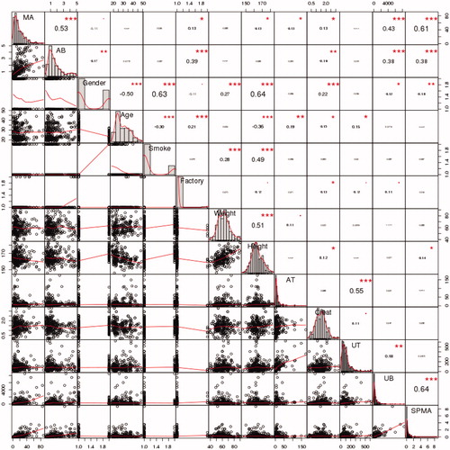
Figure 7. Visualizations of correlations. Upper left: Linear (Pearson’s) correlation corrgram (in color version, blue = positive correlation, red = negative, stronger correlations are darker). Upper right: Partial linear correlation corrgram. Lower left: Network visualization of linear correlations. In color version, green arcs represent positive correlations, red = negative, and thicker arcs and closer distances indicate stronger correlations. Lower right: Network visualization with polychloric correlations for binary variables.

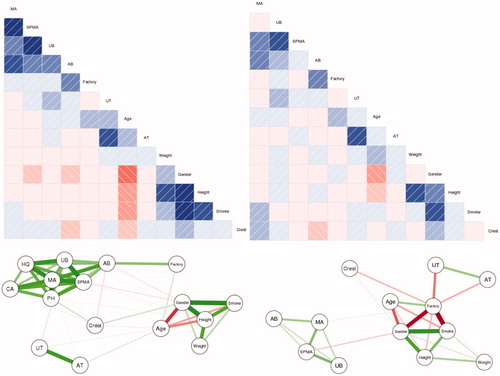
We do not base any final conclusions on the pairwise correlations in Figures 5–7, but note that age, gender, height, weight, and smoking cluster together (i.e. they are in close proximity and are joined by heavy links in Figure 7), and that air benzene (AB) and benzene metabolites often proposed as markers of benzene exposure (MA, UB, and SPMA) also cluster together (and apart from the demographic variables and the toluene variables, AT and UT). At these low concentrations, AT and UT have no significant correlations with AB and UB. This pattern is consistent with previous studies indicating that MA, UB, and SPMA are useful predictors of AB.

Partial dependence plots (PDPs)

A more thorough analysis examines how concentrations of urinary metabolites increase with increasing AB, similar to Figure 5, while controlling for (i.e. conditioning on) the values of all other variables. Such an analysis can be performed using ensembles of non-parametric models to minimize dependency on modeling assumptions (using the randomForest package in R). The top row of Figure 8 shows the resulting partial dependency plots (PDPs) for dependency of SPMA and UB, the two metabolites identified as the best markers for low-level benzene exposures, on air benzene concentration (AB) in ppm, holding other variables (Gender, Age, Smoke, Factory, Weight, Height, AT, Creat) fixed at their recorded levels for each worker. A PDP is found by averaging the predicted values of a dependent variable (benzene metabolites in Figure 8) for different values of an independent variable (AB in Figure 8), holding values of all other variables fixed. The predictions that are averaged for each value of the independent variable are made by an ensemble of machine learning predictive models or algorithms (e.g. 500 non-parametric regression trees, for the PDPs in Figure 8). For further details, see Friedman (2001). The bottom row shows PDPs for MA and HQ. (Spikes at around 3.25 ppm in the PDPs for SPMA and UB reflect outliers, i.e. exceptionally high levels of these metabolites recorded for workers with that estimated exposure concentration; this is discussed further for Figure 11.) All four PDPs show significant ordinal associations between AB and levels of each metabolite in urine (p < 0.0001 in Spearman’s rank correlation test). UB concentrations appear to increase approximately linearly with AB for AB values below 3 ppm. None of these PDPs reveals a supralinear relationship between AB levels and levels of these metabolites at low AB concentrations.

Figure 8. Partial dependence plots (PDPs) for urinary metabolites vs. air benzene (AB) concentration (ppm), controlling for Gender, Age, Smoke, Factory, Weight, Height, AT, Creatinine. PDPs were generated by the CAT software (http://cox-associates.com:8899/), which uses the randomForest package in R. (https://cran.r-project.org/web/packages/randomForest/randomForest.pdf).

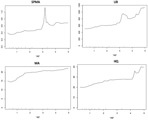
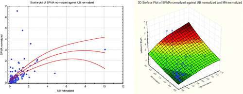
Different metabolites are best for predicting different outcomes. For example, SPMA is the best single predictor for UB, but MA is the best single predictor for AB (as measured by increase in mean squared prediction error in randomForest if each variable is omitted). Unsurprisingly, better predictions than for any single predictor can usually be achieved by using sets of several other variables to predict a dependent variable of interest. For example, for the specific task of estimating AB concentration from urinary metabolites, the pair of metabolites MA and UB is much more informative than the pair MA and SPMA, as illustrated in Figure 9.

Figure 9. Air benzene contours show that air benzene can be predicted better from MA and UB (right side) than from MA and SPMA (left side).

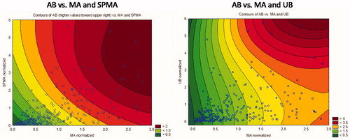
The left side of Figure 9 shows contours of equal AB (increasing from lower left to upper right) for different pairs of MA and SPMA values, and the right side shows a similar contour plot for AB given values of MA and UB. (For ease of comparison, we use the normalized values of SPMA, MA, and UB, i.e. axes are scaled so that 1 is the mean value of the corresponding variable.) The color keys show that the right-side diagram (MA and UB) has double the resolution of the left-side diagram (MA and SPMA), with contours ranging from 0.5 to 4 instead of 0 to 2 for AB concentrations. However, these diagrams show that, at low MA values, UB has little predictive power (the AB contours are nearly vertical, indicating that AB is almost independent of UB at these low AB concentrations, perhaps because UB at these low levels of AB comes mainly from other sources), whereas SPMA has better predictive power at lower MA values.

Bayesian network (BN) analysis

To obtain the best possible prediction of a variable, of course, it is necessary to condition on information from multiple variables that are informative about it. This can be done conveniently using Bayesian network (BN) methods. Figure 10 shows the structure of a BN model learned from the Tianjin data (with the knowledge-based constraint that AB should be an input). (This BN can be replicated using the CAT software at http://cox-associates.com:8899/ or the underlying bnlearn package in R using the default (hill-climbing) learning algorithm.) In this BN, two variables are informative about each other (i.e. not conditionally independent of each other, given the values of other variables, at least as far as the BN-learning can determine via statistical tests for conditional independence) if and only if they are joined by an arrow. The conditional probability distribution of each variable is determined by the values of the variables to which it is directly connected, and, given their values, is conditionally independent of the values of all other variables.

Figure 10. A Bayesian Network (BN) model learned from the Tianjin data. Arrows connect pairs of variables that are identified as being informative about (i.e. help to predict) each other.

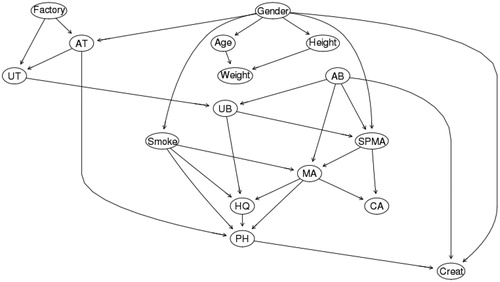
Unlike the exploratory correlation networks in Figure 7, the BN is fully non-parametric (with no assumptions of linear or ordered relations or normally distributed error terms) and multivariate (the conditional probability distribution of each variable can be conditioned on the observed or assumed values of any number of other variables). Although Gender, Height, Age, and Weight are still clustered in the BN, as are the metabolites, the BN summarizes the joint distribution of all the variables, and thus contains far more information than the corresponding pairwise correlations. It reveals patterns not obvious from correlations alone, such as a slight positive relation between UT and UB, holding AB and other variables fixed. It can be used to automatically compute the subsets of variables (“adjustment sets”) that should be conditioned on to estimate direct causal impacts of changes in one variable, such as AB, on changes in another, such as SPMA, MA, or UB (Cox 2018). For example, to estimate the causal PDP for the direct effect of AB on SPMA, any of the three adjustment sets {Gender, UB}, {AT, Factory, UB}, or {UB, UT} can be conditioned on to remove potential confounding. Any of these choices produces an estimated causal PDP very similar to the one in the upper left of Figure 8. For each of the metabolites SPMA, UB, MA, and HQ, the causal PDPs calculated from the BN are very similar to the PDPs in Figure 8, with no indication of supralinearity at low doses.

Inter-individual heterogeneity in benzene metabolism

Figure 1 shows that metabolism of benzene depends on several enzymes. Inter-individual differences in enzyme activity levels – possibly due to differences in genetic polymorphisms, lifestyle factors (e.g. alcohol consumption), or other causes – can lead to substantial differences in benzene metabolism across individuals, as reflected in the very wide variability of metabolite production across workers exposed to the same levels of air benzene (AB) (Figure 5). The potential roles of gene polymorphisms (especially those affecting NQO1 (NADPH quinone oxidoreductase), CYP2E1, MPO, GSTM1, and GSTT1 genes and activity levels) have been much discussed in literatures on inter-individual variability in susceptibility to benzene exposures in humans and rodents. Although polymorphism data are often notoriously difficult to interpret reliably, due in part to multiple testing biases and latent (unobserved) covariates, both animal and human data have been interpreted as suggesting increased production of toxic metabolites associated with specific polymorphisms (Carbonari et al. 2016; Carrieri et al. 2018). For example, mouse data have led to the conclusion that NQO1 deficiency results in sex-specific increases in benzene toxicity, as assessed by induction of micronuclei in peripheral blood cells (Bauer et al. 2003). For human data, SPMA levels of men working in a chemical plant who had GSTT1-positive genotype were reported to be significantly higher than those of subjects with GSTT1-deficient genotype (p = 0.041) (Lin et al. 2008). Petrochemical plant employees with null GSTT1 or both null STT1 and GSTM1 genotypes had significantly reduced platelets, higher leukocyte (white blood cell) counts, and higher risks of hematological disorders than other employees (Nourozi et al. 2018).

Our data set for the Tianjin factory workers lacks polymorphism information, precluding a direct examination of how they might affect benzene metabolism. Yet, the extent of inter-individual heterogeneity in benzene metabolism among Tianjin factory workers exposed to low concentrations (<5 ppm) can be illuminated by statistical analyses. Clustering can be used to identify distinct “types” (clusters) of workers, defined by different patterns of metabolite production in response to AB, even though we cannot identify specific underlying polymorphisms or other unmeasured factors that determine these types. Figure 11 shows Individual Conditional Expectation (ICE) plots (Goldstein et al. 2015) for the production of SPMA, MA, UB, and HQ by workers as functions of AB concentration (as predicted by a randomForest analysis). Each of these ICE plots characterizes inter-individual heterogeneity by partitioning workers into 3 clusters based on their predicted AB-metabolite production functions. In contrast to PDPs showing how the average value of a dependent variable (e.g. quantity of a urinary metabolite) varies with an explanatory variable (e.g. AB in ppm), holding other variables at fixed values, an ICE plot disaggregates the average response by considering individual worker-level predictions, and then reaggregating them into distinct clusters for purposes of visualization (Goldstein et al. 2011). Figure 11 shows ICE plots for the four metabolites (SPMA, UB, MA, HQ) in Figure 8, using (by default) 3 clusters in each plot to explore potential heterogeneity. The proportion of workers in each cluster is indicated in the “Prop.” box in the upper left of each plot. The clusters in Figure 3 suggest that a relatively small proportion (4%) of workers produces more UB and MA on average (light green lines) than do other workers when exposed to higher AB concentrations (e.g. at AB = 4 ppm).

Figure 11. Individual Conditional Expectation (ICE) Plots for Production of Urinary Metabolites from Low Levels of Air Benzene Exposure (AB). Fraction of worker population in each cluster is given by “Prop.” (proportion) key in the upper left of each diagram. Vertical axes are scaled to show deviations from the overall population mean value. (Plots were generated by the CAT software using the ICEbox package in R (Goldstein et al. 2015). Plots control for individual Gender, Age, Smoke, Factory, Weight, Height, and AT by conditioning on their values in random forest analysis.

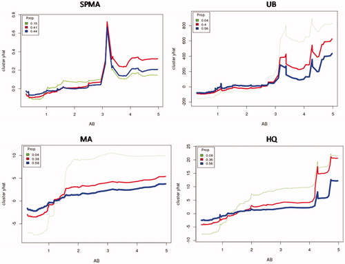
Although ICE plots are useful for exploring potential interindividual variability in exposure–response relationships, they can be sensitive to random anomalies in the data, and care is needed to obtain stable, useful clusters, e.g. by trying out different numbers of clusters and comparing how well they separate individuals (Rousseeuw 1987). We use 3 clusters throughout for exploration, without trying to further optimize clusters or filter out data anomalies. For example, the conspicuous spike in SPMA in all three clusters in the upper left panel of Figure 8 reflects the coincidence of three separate individuals with relatively high SPMA levels at around the same value of AB (3.2 to 3.4 ppm), together with the fact that regression trees discretize continuous variables and estimated values of dependent variables, leading to artificially sharp peaks around clusters of outliers compared to methods that smooth by averaging over many nearby values (e.g. spline and kernel regression methods). However, despite such artifacts, the main finding from Figure 11 is that none of the clusters for any of the metabolites exhibits supralinearity at low concentrations; thus, exploring inter-individual variability via ICE plots does not call into question the finding from the average partial dependence plots (PDPs) in Figure 8 that, for the Tianjin workers, there is no evidence of low-concentration supralinearity in production of any of the measured urinary metabolites.

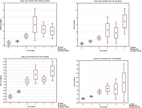
Figure 12 provides a more direct description of observed heterogeneity, without attempting to hold other factors fixed. In this plot, benzene exposure concentrations are rounded to the nearest whole number of ppm (0–5). For each of these 6 groups of AB concentrations, mean metabolite levels (dots) and standard deviations (1 sd for the boxes, 2 sd for the whiskers) are displayed. Although this visualization does not capture the skewness of the underlying metabolite distributions (see histograms in Figure 6), it does show that there is substantial inter-individual variability in metabolites produced by different individuals from approximately the same benzene exposure concentrations. The shapes of the plots at the lowest concentrations also show sub-linearity, i.e. the increases in metabolites produced are greater when AB increases from 1 to 2 than when it increases from 0 to 1.

Figure 12. Categorized box-and-whisker plots show substantial interindividual variability in production of urinary metabolites (clockwise from upper left: normalized SPMA, UB, MA, HQ values, scaled so that population mean = 1 for each metabolite). Metabolite production is sub-linear at low doses (AB < 3 ppm) (i.e. successive increases in AB by 1 unit generate larger increases in metabolites).

Figure 13 depicts the joint values of multiple urinary metabolites (UB and SPMA on the left, with a quadratic regression model (solid curve) and 95% normal confidence intervals shown as dashed curves superimposed on the scatterplot to give a heuristic visual impression of how these variables co-vary, although either could be chosen as the dependent variable for this purpose; and with UB, SPMA, and MA on the right), for workers exposed to 1 ppm of AM (rounded to the nearest ppm). These scatterplots not only illustrate the inter-individual variability in metabolite levels for approximately the same AB exposure, but they also show that a few individuals have much higher levels of benzene metabolites than others. This interindividual variability is too great to be well modeled by a regression curve with a normally distributed, exposure-independent, additive error term. This highlights the value of using non-parametric methods, as in Figures 8–11, to understand the conditional distributions of metabolites given AB levels.

Figure 13. Joint scatter plots for SPMA and UB (left) and MA, UB, and SPMA (right) for workers exposed to 1 ppm (rounded to the nearest ppm) of benzene in air (AB = 1).

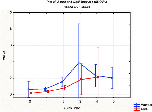
Consistent with earlier studies (Tranfo et al. 2018), Figure 14 shows that women produce slightly more SPMA than men at low benzene concentrations; this explains the arrow from Gender to SPMA in the BN in Figure 10. However, the effect of gender on metabolism is small compared to other inter-individual differences, as reflected in the wide vertical spread of metabolite levels for approximately the same AB concentrations (Figure 12).

Figure 14. Women (upper curve) produce more SPMA than men at low concentrations (AB < 3 ppm) Vertical bars indicate approximate 95% confidence intervals.

Intra-individual variability in benzene metabolism

The Tianjin factory worker contains repeated measurements of benzene exposure concentrations and urinary metabolite levels for some individual workers, with 263 data records for 177 individual workers. There were 4 measurement days (records in the data set) for 2 of the workers with low AB concentrations (<5 ppm); 3 records for each of another 11 of these workers; 2 records for 58 workers; and a single record for each of the remaining 106 workers. The repeated measurements provide an opportunity to study within-individual variability in exposure and metabolism. The previous analyses treated each measurement of metabolites in an individual on a day as a data point, without attempting to model possible correlations among data points from the same individual on different days. (Dropping repeated measurements on the same individuals does not change the conclusions we have drawn, for reasons explained next, but reduces the number of data points in plots from 263 5o 177.) Our nonparametric analyses have avoided making assumptions that data points or errors are independent, in part to avoid the complexity of modeling intra-individual variability and serial correlations, but we now examine the stability of repeated measurements in individuals over time.

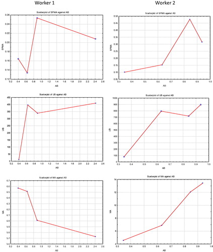
Figure 15 plots the levels of SPMA, UB, and MA (top, middle, and bottom rows, respectively) at different AB levels, for the 2 individuals with 4 measurements each. (Note the very different vertical scales for metabolites in these plots.) Worker 2 (right side) has close to twice the peak metabolite levels of Worker 1 (left side) for each metabolite, even though Worker 1 has a higher maximum benzene exposure concentration (2.4 ppm instead of less than 1 ppm). However, neither individual has uniformly higher levels of metabolites than the other across all four repeated measurements and AB levels (although Worker 2 does have higher levels of UB than Worker 1, even at lower AB exposures). While a study of only 2 individual workers with 4 repeated measurements each does not permit confident generalizations about intra-individual variability in benzene metabolism, the types of variability illustrated in Figure 15 (including some curves in which metabolites decrease as AB increases, as in the slight decrease in MA shown in the lower left of Figure 15) also occur for the 11 workers with 3 repeated measurements each. However, the effects of intra-individual variability in metabolism are difficult to discern, since the workers received different air benzene concentrations on different days. Despite these limitations, Figure 14 suggests that, for the worker with relatively high metabolite formation (Worker 2), the levels of all three metabolites were much more than twice as great at AB concentrations between 0.8 ppm and 1 ppm (two right-most points in each plot) as at AB concentrations of about 0.35 ppm (leftmost point in each plot).

Figure 15. Urinary metabolites vs. AB (ppm) for 2 Individual Workers, each with 4 Repeated Measurements. (Top row SPMA; middle row UB; bottom row MA).

Levels of benzene metabolites and markers in relation to increased health risks

Average levels of urinary benzene metabolites increase with increasing AB exposure in the population of Chinese factory workers exposed to relatively low concentrations of benzene in air (AB < 5 ppm), even though there is considerable inter-individual variability in the quantity of metabolites formed for any given level of AB (Figure 12). The question of what levels of metabolites (or of other markers with which they are correlated, such as 8-OHdG, various adducts, or micronuclei induction in peripheral blood lymphocytes) correspond to increased risk of MDS and AML has been much debated, with substantial differences in conclusions. For example:

• Vlaanderen et al. (2010) fit non-parametric (spline) smooth curves to heterogeneous data from 9 human studies of estimated cumulative benzene exposures and leukemia. They concluded that the best-fitting curves were linear or super-linear at low exposures, and that there was significantly increased risk of leukemia [relative risk (RR) = 1.14; 95% confidence interval (CI), 1.04–1.26] at estimated exposure levels as low as 10 ppm-years. Although these analyses did not adjust for errors in exposure estimates and did not address peak exposures, they are generally consistent both with earlier studies that found no threshold for estimated cumulative benzene exposures associated with increased risk of AML and other diseases (Glass et al. 2003) and also with subsequent reviews that accept the plausibility of leukemogenic effects of benzene even at low cumulative exposures, such as 0.5 ppm-years (Yoon et al. 2018).

• By contrast, Schnatter et al. (2012) combined data from 3 nested case–control studies of petroleum distribution workers from Australia, Canada, and the United Kingdom, and estimated that risk of MDS, but not of AML or other leukemias or myeloproliferative disorders, increased substantially (estimated odds ratio in a conditional logistic regression model was OR = 4.33) for workers with estimated cumulative benzene exposures >2.9 ppm-years compared to workers with estimated cumulative benzene exposures <0.35 ppm-years (highest vs. lowest tertiles, respectively). MDS risk was increased specifically in workers with estimated peak exposures >3 ppm. However, this analysis also used reconstructed exposures with unknown errors, and the error distributions were not modeled, potentially leading to misestimates of the true peak exposure concentrations that are associated with increased MDS risk. The authors suggest that MDS, rather than AML or other endpoints, may be the most relevant health risk at relatively low exposure concentrations.

The analyses in this paper suggest a different perspective from either of these on the human health risks caused by low exposure concentrations of benzene, as follows.

• If risk of benzene-induced diseases depends on chronic inflammation in the bone marrow (perhaps mediated by activation of the NLRP3 inflammasome) (Sallman and List 2019), then cumulative exposure (ppm-years) is not an adequate dose metric for predicting risk. Instead, risk over a lifetime depends on when (i.e. at what age) chronic inflammation is induced, which in turn depends on the time pattern of exposure and of reactive metabolites reaching the marrow at sufficiently high and prolonged concentrations to cause inflammation. On the relatively long time scale of a lifetime, the details of exposure time patterns that lead to chronic inflammation of target tissues may be relatively unimportant compared to the age at which chronic inflammation begins.

• PBPK models imply that, for a steady administered concentration of air benzene (AB), concentrations of metabolites in bone marrow increase over time until a dynamic equilibrium level is reached at which the rate of each metabolite’s removal equals the rate of its addition to the marrow (via distribution from the liver and via local metabolism in the marrow). If exposure concentration of benzene in inhaled air is low enough, then the dynamic equilibrium concentration will be below the inflammasome activation threshold (or the smallest such threshold, if values are heterogeneous). Inflammation, and resulting inflammation-mediated increases in MDS and other disease risks, will not be triggered, and extending the duration of such a low-level exposure increases cumulative exposure (ppm-years) without increasing risk. It is not necessary to know which toxic metabolite(s) are involved in the pathogenesis of MDS and AML to reach this qualitative conclusion.

• Conversely, if the PBPK dynamic equilibrium for a given AB concentration is only slightly below the activation threshold, then twice this concentration administered for half as many years might quickly trigger inflammation, even though the original exposure (with the same ppm-years) did not. Cumulative exposure received after chronic inflammation starts may be nearly irrelevant if the chronic inflammation itself dominates subsequent risk.

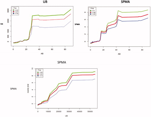
• Even if inflammation is not the rate-limiting key event for increasing risk of MDS and AML, cumulative exposure is still a highly misleading metric for realistic past exposures involving AB concentrations in excess of about 20 ppm. Although we have focused so far on workers exposed to <5 ppm, Figure 16 shows a wider perspective by plotting UB (in nM) and SPMA (μM) against AB for each of three clusters of workers in an individual conditional expectation (ICE) plot. The differences in metabolite production that we have been examining for AB < 5 ppm are almost negligible, on this expanded scale, compared to the main pattern of approximately linear metabolism at AB concentrations below about 15 ppm and a steep increase in production per unit of AB above that level, for all three clusters (light, medium, and heavy metabolizers). (As in Figure 11, these ICE plots also use 3 clusters by default, and no effort was made to further optimize the default clustering, but the major pattern of approximately linear metabolite production at low concentrations is robust and holds also for the aggregate data without clustering, analogous to Figure 8.) The S-shaped pattern shown for urinary benzene (top left of Figure 16) invites speculation about possible pharmacokinetic and metabolic mechanisms, such as saturation of different pathways for forming and removing metabolites, but the PBPK models we have reviewed lack high resolution at these relatively low concentrations (Figure 3), and we leave more detailed investigation and explanation of the empirically observed patterns for future research.

• The bottom panel of Figure 16 shows that SPMA can also be predicted from UB instead of AB. If UB is used instead of AB as a predictor of SPMA (along with the other variables in Figure 16) in random forest analysis, the percentage of variance in SPMA that is explained increases from about 36% to about 41% (and to 47% if UB and AB are both used). A possible explanation is that urinary benzene (UB) reflects inter-individual variability in metabolism or in other exposure routes (e.g. dermal) that air benzene (AB) measurements do not address; differences in measurement error variances between UB and AB might also play a role.

• The steeply sub-linear (hockey-stick) functions for metabolism in the top panels of Figure 16 imply that a worker exposed to an average of 10 ppm-years consisting of 3 months a year of 40 ppm and 9 months per year of 0 ppm would have far higher average concentrations of metabolites (averaged over the year) than a similar worker exposed to 10 ppm throughout the year. Cumulative exposure and peak exposure both fail to capture the most relevant information for risk prediction, which is how long the worker spends exposed to AB concentrations sufficient to produce harmful (risk-increasing) concentrations of metabolites in the bone marrow.

Figure 16. Top: Sub-linear production of benzene metabolites (UB on left; SPMA on right) by workers (partitioned into three clusters to indicate inter-individual heterogeneity), given AB. Bottom: Prediction of SPMA from UB. (Plots control for individual Gender, Age, Smoke, Factory, Weight, Height, and AT by conditioning on their values in random forest analysis.).

From this perspective, mixed and contradictory results are to be expected from past studies and reviews that use cumulative exposure to benzene as a predictor of risk. The same cumulative exposure may be harmful or harmless, depending on how it is distributed over time.

The same reasoning implies that errors in exposure estimates can play a key role in determining the risk attributed to a given average exposure concentration. For example, the data and BN model predictions of Hack et al. (2010) indicate that AML risk increases for benzene concentrations above a level estimated as between 1 ppm and 10 ppm. For workers with occasional exposures to concentrations above 25 ppm, but estimated average exposures between 1 and 10 ppm, the risk may be dominated by metabolites formed during occasional exposures to higher concentrations (Figure 16), although it is attributed to the lower average exposure concentrations. These considerations, if correct, imply that many previous analyses of benzene dose–response that use estimated cumulative exposure (ppm-years) to predict AML or MDS risk, without characterizing variability of exposure concentrations around their estimated values, lose essential information on which risk depends. Figure 16 suggests that a better understanding of benzene-associated risk can be achieved by considering the fraction of a worker’s time spent exposed to relatively high concentrations (e.g. AB > 15 ppm), as this may dominate the contribution of exposure to formation of toxic metabolites.

How much practical difference does the claimed supralinearity make for benzene risk analysis?

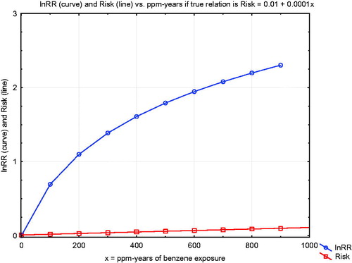
This review of aspects of benzene metabolism and health risks reviewed was motivated by a concern that supralinear exposure–response relationships for benzene, if they are real, could suggest that regulatory approaches to protecting workers by limiting exposure concentrations and durations might be inadequate: “The policy implications of these studies are staggering. In theory, they indicate that regulatory agencies should strive to achieve near-zero exposures… to protect people’s health” (Lanphear 2017). Our main conclusion is that none of the evidence we have reviewed suggests supralinearity, and some suggests that there are exposure concentrations below which health risks are not expected to occur. To put this qualitative conclusion into a more quantitative perspective, Figure 17 reproduces the original figure from Vlaanderen et al. (2010) supporting claims of supralinear exposure–response relationships for benzene (Lanphear 2017). The vertical axis shows the natural logarithm of the relative risk ratio (i.e. the ratio of estimated risk at each cumulative exposure level, in ppm-years, to the risk without exposure).

Figure 17. Comparison of linear and supralinear (spline) curves for lnRR vs. ppm-years of exposure, from Vlaanderen et al. (2010).

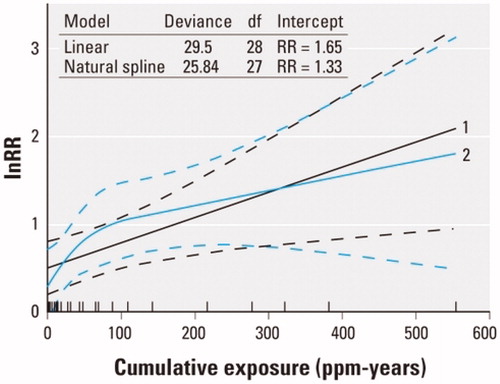
Thus, a value of 3 on the vertical axis corresponds to a relative risk ratio of e³ = 20. As the authors explain, “Natural spline models…as well as linear models were fitted to the data to investigate the shape of the exposure–response relation. To improve the statistical properties of the regression models, we fitted all models to the natural logarithm of the reported risk estimates.” They conclude that “The natural spline showed a supralinear shape at cumulative exposures less than 100 ppm-years, although this model fitted the data only marginally better than a linear model (p = 0.06).” For a risk manager, Figure 17 seems to suggest that model 2 (the “supralinear” model) implies much steeper risk-reduction benefits from reducing ppm-years of benzene exposure to zero than does model 1 (linear). However, this apparent implication reflects an algebraic illusion created by use of a log-transformed relative risk ratio: such a transformation creates a “supralinear” curve (for lnRR) even if the exposure–response relationship for absolute risk is linear, as our review suggests is the case. To clarify this algebraic point, Figure 18 plots both a hypothetical linear exposure–response relationship, Risk = 0.01 + 0.0001*(ppm-years), and the corresponding log-transformed relative risk ratio, on the same axes. The latter curve is “supralinear” even though absolute risk is known to increase linearly with cumulative exposure. Such a transformed curve provides no evidence of “staggering” policy implications that reducing cumulative exposure creates disproportionately large risk-reduction benefits at low exposure concentrations. Such a misinterpretation confuses an algebraic transformation with a real-world effect. As a practical matter, the linear and “supralinear” models in Figure 1 fit the data approximately equally well, and neither implies a departure from linearity of the estimated absolute risk-vs.-cumulative exposure curve at low concentrations.

Figure 18. “Supralinearity” for lnRR is compatible with a linear exposure–response function.

Conclusions

Recent literature has raised the question of whether dose–response relationships for benzene are supra-linear, creating disproportionately high risks per ppm-year of exposure for exposure concentrations below 1 ppm (Rappaport et al. 2010; Lanphear 2017). We have examined this hypothesis using findings from recent literature on mode of action (MoA) and mechanistic considerations for benzene-induced myelodysplastic syndrome (MDS) and acute myeloid leukemia (AML) and by applying modern data science techniques to quantify and visualize relationships between air benzene and production of toxic metabolites in previously studied data for Tianjin factory workers. Our main conclusions from these analyses are as follows:

1. Physiologically based pharmacokinetics (PBPK) modeling predicts that production of toxic metabolites, and their levels in both circulating blood and in urine, are approximately linear (i.e. proportional to benzene concentration in inhaled air), or mildly sublinear, at low exposure concentrations (Figure 3). These models and the data sets used to build and validate them provide no evidence of supralinearity.

2. Bayesian network (BN) modeling also suggests a sublinear (J-shaped) relationship between estimated air benzene (AB) concentrations and AML risk (Hack et al. 2010).

3. Data for Tianjin workers shows approximately linear metabolism at low concentrations (AB < 5 ppm), i.e. production of urinary metabolites is approximately proportional to concentration of benzene in inhaled air (Figure 5). This linearity holds over nearly 2 orders of magnitude, from the lowest measured concentrations (about 0.2 ppm) to well over 10 ppm. At concentrations below 3 ppm, the production of metabolites is mildly sublinear (Figure 12). This is not inconsistent with previous claims of supralinear relationships in meta-analyses that have considered the logarithm of relative risk (lnRR) as the dependent variable (Vlaanderen et al. 2010; Lanphear 2017), since a linear exposure–response relationship implies a supralinear exposure-lnRR relationship (Figure 18).

4. The production of metabolites at higher AB concentrations increases disproportionately before becoming saturated (Figure 16). This implies that cumulative exposure (ppm-years) is not a sufficient summary of exposure from which to predict risk, which may help to explain conflicting conclusions in the literature.

5. The steeply sublinear shape (“elbow”) at the left end of the metabolite-vs. AB curve (Figure 16) also makes it important for risk assessments to consider the variability of exposure concentrations around estimated exposure concentrations. Analyses in which a mix of relatively high (e.g. AB > 15 ppm) and low (e.g. AB < 10 ppm) concentrations are summarized in a single cumulative exposure (ppm-year) estimate for each worker are likely to over-estimate low-concentration risk, by attributing to them adverse effects that are created primarily by the high concentrations.

6. Although there is substantial interindividual variability in levels of urinary metabolites of benzene produced at air benzene concentrations above about 3 ppm, the variability is much less at lower concentrations (Figure 12). For example, an air benzene concentration that does not exceed 1 ppm would keep even the upper ends of the worker population distribution of metabolite levels (the top “whiskers” in the box- and-whisker plots in Figure 12) below current mean levels (normalized to 1 in Figure 12). If adverse health effects occur primarily among people with above-average levels of some of these metabolites, then it would be practical to protect this population by keeping measured AB < 1ppm, even taking into account interindividual variability in benzene metabolism. However, our dataset does not contain adverse outcome endpoints, so we cannot estimate health-protective time-weighted averages and short-term exposure limits more precisely from these data.

7. If chronic inflammation via activation of the NLRP3 inflammasome is a critical event for induction of MDS by benzene (Sallman and List 2019), then PBPK considerations imply that sufficiently low AB concentrations will not create concentrations of toxic metabolites that exceed the NLRP3 inflammasome activation threshold, and hence they will not increase the risk of MDS, no matter how long the exposure duration is. This illustrates why ppm-years is not adequate as a predictor of risk: twice the ppm for half as many years might cause MDS even if lower concentrations for longer do not. More generally, the same ppm-years number can be harmless or harmful, depending on how AB concentrations are distributed over time; this general point holds for a variety of mechanisms involving tissue damage and repair, whether or not they involve inflammation (Rhomberg 2009). The hypothesis of a threshold below which no excess risk occurs is consistent with plots of epidemiological data from multiple studies showing no clear upward trend in leukemia risk with exposures below 20 ppm-years (Vlaanderen et al. 2010, Figure 1(b)), but the limitations we have noted for ppm-years as an exposure metric make it difficult to interpret such data or to identify clear concentration thresholds that might be tied to NLRP3 inflammasome activation, depletion of antioxidant pools, or other threshold mechanisms; this appears to be a worthwhile area for future research.

8. If MDS is the most sensitive adverse health effect endpoint at relatively low exposure concentrations (Schnatter et al. 2012), then an exposure concentration threshold may exist for increases in risk due to benzene exposure. However, the use of cumulative exposures and reconstructed (uncertain) exposure estimates would obscure any such threshold. In addition, the substantial inter-individual variability in benzene metabolism (Figures 11–14) implies that any exposure concentration threshold for AB has a distribution in a worker population.

These points distinguish among three potential sources of nonlinearity in estimated exposure–response relationships: nonlinear biological mechanisms (such as an inflammasome activation threshold or metabolic saturation); empirical patterns in outcomes (observations of metabolites and biomarkers in actual populations, with techniques such as Bayesian network analysis applied to control for potential confounding and extraneous factors); and mathematical modeling assumptions and transformations used in statistical curve-fitting (Figures 17 and 18). Previous sections have illustrated how reported pharmacokinetic and pharmacodynamic mechanisms, Bayesian networks, and empirical exposure–response models can be viewed and at least partly integrated and understood from these three perspectives. The main insight from these different perspectives is that if a dose–response relationship is truly supralinear, then there should be causal biological mechanisms in the pharmacokinetics (PK) or pharmacodynamics (PD) that explain it, and plotting data on untransformed axes (i.e. plotting absolute risk or its causal predecessors, such as reactive metabolites, against exposure) should show the supralinear pattern. The PK and PD mechanisms and data we have reviewed for benzene support linearity or sublinearity at low exposure concentrations, with quantitative risks and metabolite levels at low concentrations no higher (but possibly considerably lower) than would be expected by extrapolating risks measured at higher exposures linearly down to zero (Figure 8, Hack et al. 2010). These conclusions are consistent with previous general conceptual frameworks and models of the effects of time patterns of administered concentrations of inhaled toxicants on the amounts of time that target tissue concentrations spend above thresholds needed to induce damage (Rhomberg 2009).

Although the data and MoA literature we have examined do not support a hypothesis of supralinearity of risks at low benzene concentrations, they do suggest opportunities to improve benzene risk assessments by focusing on the proportion and timing of low and high exposure concentrations in each worker’s exposure history, rather than combining these into a single cumulative exposure metric, consistent with some previous recommendations for modeling inhaled toxicants in general (Rhomberg 2009). For practical methods, pharmacokinetic (PBPK) modeling or PDP curves (such as Figure 16) can be used to convert time series of approximate exposure concentrations to corresponding time series of corresponding benzene metabolites. Identifying the time until inflammation is triggered, and using Bayesian networks developed from data (Figure 10) to estimate increases in risk during periods of increased inflammatory markers, while controlling for other observed variables (e.g. age, sex, smoking, diet, polymorphisms, and other markers if available) appears to be a promising and practical approach for using current data science methods to advance benzene risk modeling. A potentially important risk management implication is that maintaining blood concentrations of benzene and its metabolites below levels that cause inflammation or other damage can protect workers against adverse effects of benzene. In this case, smaller concentrations (and durations) are expected to be disproportionately safe rather than disproportionately dangerous (Rhomberg 2009).

Acknowledgements

The authors thank three anonymous reviewers and Roger McClellan, who closely read an earlier version and made very substantive and constructive suggestions for improving the exposition. Figures 17 and 18 and the accompanying discussion were added in the course of revising the paper in response to reviewer comments. This paper was cleared for publication by both Concawe and ExxonMobil without changes to its content.

Declaration of interest

The authors disclosed receipt of the following financial support for the research, authorship, and/or publication of this article. Dr. Cox’s time for development of the risk modeling approach reported here and drafting the paper was supported by the following contract research projects undertaken by his employer, Cox Associates LLC: (1) A 2019–2020 research contract with Concawe, a division of the European Petroleum Refiners Association, to review low-dose benzene metabolism and its implications for the shapes of dose–response functions and human health risk assessment. Concawe members range from multi-national oil and gas Companies that operate in exploration and production, refining, and chemicals, to European regional and National Companies operating one or more refineries in the European Union. (2) A 2015 research collaboration with the George Washington University Regulatory Studies Center, funded by ExxonMobil, to develop the Causal Analytics Toolkit (CAT) software used to perform the machine learning analyses described in this work. All aspects of this article, including the research questions addressed, the methods developed and applied, and the conclusions reached, are solely the authors’. The other authors were granted time by their employers to work on this paper as part of their research for Concawe on health risk analysis. None of the authors has engaged in any legal, regulatory, or advocacy activities in the last decade related to the contents of this paper, although Dr. Cox has advocated for use of causal analysis and methods such as Bayesian network analysis in risk analysis outside the specific context of benzene.

References

- Anderson LA, Pfeiffer RM, Landgren O, Gadalla S, Berndt SI, Engels EA. 2009. Risks of myeloid malignancies in patients with autoimmune conditions. Br J Cancer. 100:822–828.
- Arnold SM, Angerer J, Boogaard PJ, Hughes MF, O'Lone RB, Robison SH, Schnatter AR. 2013. The use of biomonitoring data in exposure and human health risk assessment: benzene case study. Crit Rev Toxicol. 43:119–153.
- Bauer AK, Faiola B, Abernethy DJ, Marchan R, Pluta LJ, Wong VA, Roberts K, Jaiswal AK, Gonzalez FJ, Butterworth BE, et al. 2003. Genetic susceptibility to benzene-induced toxicity: role of NADPH: quinone oxidoreductase-1. Cancer Res. 63:929–935.
- Bechtold WE, Henderson RF. 1993. Biomarkers of human exposure to benzene. J Toxicol Environ Health. 40:377–386.
- Bogen KT. 2019. Inflammation as a cancer co-initiator: new mechanistic model predicts low/negligible risk at noninflammatory carcinogen doses. Dose Response. 17:1559325819847834.
- Campagna M, Satta G, Campo L, Flore V, Ibba A, Meloni M, Tocco MG, Avataneo G, Flore C, Fustinoni S, et al. 2012. Biological monitoring of low-level exposure to benzene. Med Lav. 103:338–346.
- Carrieri M, Spatari G, Tranfo G, Sapienza D, Scapellato ML, Bartolucci GB, Manno M. 2018. Biological monitoring of low level exposure to benzene in an oil refinery: effect of modulating factors. Toxicol Lett.
- Carbonari D, Chiarella P, Mansi A, Pigini D, Iavicoli S, Tranfo G. 2016. Biomarkers of susceptibility following benzene exposure: influence of genetic polymorphisms on benzene metabolism and health effects. Biomark Med. 10:145–163.
- Cox LA Jr. 1995. Simple relations between administered and internal doses in compartmental flow models. Risk Anal. 15:197–204.
- Cox LA, Schnatter AR, Boogaard PJ, Banton M, Ketelslegers HB. 2017. Non-parametric estimation of low-concentration benzene metabolism. Chem Biol Interact. 278:242–255.
- Cox LA Jr. 2018. Modernizing the Bradford Hill criteria for assessing causal relationships in observational data. Crit Rev Toxicol. 48:682–712.
- Cox LAT Jr. 2019. Risk analysis implications of dose-response thresholds for NLRP3 inflammasome-mediated diseases: respirable crystalline silica and lung cancer as an example. Dose Response. 17:155932581983690.
- Das M, Chaudhuri S, Law S. 2012. Benzene exposure – an experimental machinery for induction of myelodysplastic syndrome: stem cell and stem cell niche analysis in the bone marrow. J Stem Cells. 7:43–59.
- Du X, Jiang S, Zeng X, Zhang J, Pan K, Song L, Zhou J, Kan H, Sun Q, Zhao J, et al. 2019. Fine particulate matter-induced cardiovascular injury is associated with NLRP3 inflammasome activation in Apo E-/- mice. Ecotoxicol Environ Saf. 174:92–99.
- Friedman JH. 2001. Greedy function approximation: a gradient boosting machine. Ann Statist. 29:1189–1232.
- Fustinoni S, Campo L, Mercadante R, Consonni D, Mielzynska D, Bertazzi PA. 2011. A quantitative approach to evaluate urinary benzene and S-phenylmercapturic acid as biomarkers of low benzene exposure. Biomarkers. 16:334–345.
- Galbraith D, Gross SA, Paustenbach D. 2010. Benzene and human health: a historical review and appraisal of associations with various diseases. Crit Rev Toxicol. 40 Suppl 2:1–46.
- Glass DC, Gray CN, Jolley DJ, Gibbons C, Sim MR, Fritschi L, Adams GG, Bisby JA, Manuell R. 2003. Leukemia risk associated with low-level benzene exposure. Epidemiology. 14:569–577.
- Goldstein A, Kapelner A, Bleich J, Pitkin E, 2015. Peeking inside the black box: visualizing statistical learning with plots of individual conditional expectation. J Comput Graph Stat. 24:44–65.
- Grigoryan H, Edmands WMB, Lan Q, Carlsson H, Vermeulen R, Zhang L, Yin SN, Li GL, Smith MT, Rothman N, et al. 2018. Adductomic signatures of benzene exposure provide insights into cancer induction. Carcinogenesis. 39:661–668.
- Gross SA, Paustenbach DJ. 2018. Shanghai Health Study (2001–2009): what was learned about benzene health effects? Crit Rev Toxicol. 48:217–251.
- Guo X, Zhong W, Chen Y, Zhang W, Ren J, Gao A. 2019. Benzene metabolites trigger pyroptosis and contribute to haematotoxicity via TET2 directly regulating the Aim2/Casp1 pathway. EBioMedicine. 47:578–589.
- Hack CE, Haber LT, Maier A, Shulte P, Fowler B, Lotz WG, Savage RE Jr. 2010. A Bayesian network model for biomarker-based dose response. Risk Anal. 30:1037–1051.
- Hamling JS, Coombs KJ, Lee PN. 2019. Misclassification of smoking habits: an updated review of the literature. World J Meta-Anal. 7:31–50.
- Hirabayashi Y, Inoue T. 2010. Benzene-induced bone-marrow toxicity: a hematopoietic stem-cell-specific, aryl hydrocarbon receptor-mediated adverse effect. Chem Biol Interact. 184:252–258.
- Hornung RW, Lanphear BP. 2014. The supralinear dose-response for environmental toxicants: a statistical artifact? Clin Toxicol (Phila). 52:88–90.
- Kerzic PJ, Irons RD. 2017. Distribution of chromosome breakpoints in benzene-exposed and unexposed AML patients. Environ Toxicol Pharmacol. 55:212–216.
- Knutsen JS, Kerger BD, Finley B, Paustenbach DJ. 2013. A calibrated human PBPK model for benzene inhalation with urinary bladder and bone marrow compartments. Risk Anal. 33:1237–1251.
- Lanphear BP. 2017. Low-level toxicity of chemicals: no acceptable levels? PLoS Biol. 15:e2003066.
- Lin LC, Chen WJ, Chiung YM, Shih TS, Liao PC. 2008. Association between GST genetic polymorphism and dose-related production of urinary benzene metabolite markers, trans, trans-muconic acid and S-phenylmercapturic acid. Cancer Epidemiol Biomarkers Prev. 17:1460–1469.
- McHale CM, Zhang L, Smith MT. 2012. Current understanding of the mechanism of benzene-induced leukemia in humans: implications for risk assessment. Carcinogenesis. 33:240–252.
- McNally K, Sams C, Loizou GD, Jones K. 2017. Evidence for non-linear metabolism at low benzene exposures? A reanalysis of data. Chem Biol Interact. 278:256–268.
- Meek ME, Klaunig JE. 2010. Proposed mode of action of benzene-induced leukemia: Interpreting available data and identifying critical data gaps for risk assessment. Chem Biol Interact. 184:279–285.
- Neumann HG. 2009. Risk assessment of chemical carcinogens and thresholds. Crit Rev Toxicol. 39:449–461.
- Nourozi MA, Neghab M, Bazzaz JT, Nejat S, Mansoori Y, Shahtaheri SJ. 2018. Association between polymorphism of GSTP1, GSTT1, GSTM1 and CYP2E1 genes and susceptibility to benzene-induced hematotoxicity. Arch Toxicol. 92:1983–1990.
- Price PS, Rey TD, Fontaine DD, Arnold SM. 2012. A reanalysis of the evidence for increased efficiency in benzene metabolism at airborne exposure levels below 3 p.p.m. Carcinogenesis. 33:2094–2099.
- Qian S, Han Y, Shi Y, Xu W, Zhu Y, Jiang S, Chen Y, Yu Z, Zhang S, Yang Y, et al. 2019. Benzene induces haematotoxicity by promoting deacetylation and autophagy. J Cell Mol Med. 23:1022–1033.
- Qu Q, Shore R, Li G, Jin X, Chen LC, Cohen B, Melikian AA, Eastmond D, Rappaport S, Li H, et al. Validation and evaluation of biomarkers in workers exposed to benzene in China. Res Rep Health Eff Inst. 2003;115:1–72.
- Rappaport SM, Kim S, Lan Q, Li G, Vermeulen R, Waidyanatha S, Zhang L, Yin S, Smith MT, Rothman N. 2010. Human benzene metabolism following occupational and environmental exposures. Chem Biol Interact. 184:189–195.
- Rappaport SM, Kim S, Thomas R, Johnson BA, Bois FY, Kupper LL. 2013. Low-dose metabolism of benzene in humans: science and obfuscation. Carcinogenesis. 34:2–9.
- Rappaport SM, Kim S, Lan Q, Vermeulen R, Waidyanatha S, Zhang L, Li G, Yin S, Hayes RB, Rothman N, et al. 2009. Evidence that humans metabolize benzene via two pathways. Environ Health Perspect. 117:946–952.
- Rhomberg LR. 2009. Uptake kinetics, species differences, and the determination of equivalent combinations of air concentration and exposure duration for assessment of acute inhalation toxicity. Hum Ecol Risk Assess. 15:1099–1145.
- Richardson DB. 2009. Multistage modeling of leukemia in benzene workers: a simple approach to fitting the 2-stage clonal expansion model. Am J Epidemiol. 169:78–85.
- Rousseeuw PJ. 1987. Silhouettes: a graphical aid to the interpretation and validation of cluster analysis. J Comput Appl Math. 20:53–65.
- Rushton L, Schnatter AR, Tang G, Glass DC. 2014. Acute myeloid and chronic lymphoid leukaemias and exposure to low-level benzene among petroleum workers. Br J Cancer. 110:783–787.
- Sallman DA, Cluzeau T, Basiorka AA, List A. 2016. Unraveling the pathogenesis of MDS: the NLRP3 inflammasome and pyroptosis drive the MDS phenotype. Front Oncol. 6:151.
- Sallman DA, List A. 2019. The central role of inflammatory signaling in the pathogenesis of myelodysplastic syndromes. Blood. 133:1039–1048.
- Schnatter AR, Glass DC, Tang G, Irons RD, Rushton L. 2012. Myelodysplastic syndrome and benzene exposure among petroleum workers: an international pooled analysis. J Natl Cancer Inst. 104:1724–1737.
- Slenter DN, Kutmon M, Hanspers K, Riutta A, Windsor J, Nunes N, Mélius J, Cirillo E, Coort SL, Digles D, et al. 2018. WikiPathways: a multifaceted pathway database bridging metabolomics to other omics research. Nucleic Acids Res. 46:D661–D667.
- Smith MT. 1996. Overview of benzene-induced aplastic anaemia. Eur J Haematol Suppl. 60:107–110.
- Snyder R. 2012. Leukemia and benzene. Int J Environ Res Public Health. 9:2875–2893.
- Son MY, Deng CX, Hoeijmarkers JH, Rebel VI, Hasty P. 2016. A mechanism for 1,4-benzoquinone-induced genotoxicity. Oncotarget. 7:46433–46447.
- Teras LR, Diver WR, Deubler EL, Krewski D, Flowers CR, Switchenko JM, Gapstur SM. 2019. Residential ambient benzene exposure in the United States and subsequent risk of hematologic malignancies. Int J Cancer. 145:2647–2660.
- Titmarsh GJ, McMullin MF, McShane CM, Clarke M, Engels EA, Anderson LA. 2014. Community-acquired infections and their association with myeloid malignancies. Cancer Epidemiol. 38:56–61.
- Tranfo G, Pigini D, Paci E, Bauleo L, Forastiere F, Ancona C. 2018. Biomonitoring of urinary benzene metabolite SPMA in the general population in central Italy. Toxics. 6:37.
- Vlaanderen J, Portengen L, Rothman N, Lan Q, Kromhout H, Vermeulen R. 2010. Flexible meta-regression to assess the shape of the benzene-leukemia exposure-response curve. Environ Health Perspect. 118:526–532.
- Waddell WJ. 2006. Critique of dose response in carcinogenesis. Hum Exp Toxicol. 25:413–436.
- Wang L, He X, Bi Y, Ma Q. 2012. Stem cell and benzene-induced malignancy and hematotoxicity. Chem Res Toxicol. 25:1303–1315.
- Weisel CP. 2010. Benzene exposure: an overview of monitoring methods and their findings. Chem Biol Interact. 184:58–66.
- Wei J, Wang H, Wang H, Wang B, Meng L, Xin Y, Jiang X. 2019. The role of NLRP3 inflammasome activation in radiation damage. Biomed Pharmacother. 118:109217.
- Yokley K, Tran HT, Pekari K, Rappaport S, Riihimaki V, Rothman N, Waidyanatha S, Schlosser PM. 2006. Physiologically-based pharmacokinetic modeling of benzene in humans: a Bayesian approach. Risk Anal. 26:925–943.
- Yoon JH, Kwak WS, Ahn YS. 2018. A brief review of relationship between occupational benzene exposure and hematopoietic cancer. Ann Occup Environ Med. 30:33.