Damage tracking in laboratory reinforced concrete bridge columns under reverse-cyclic loading using fusion-based imaging

ABSTRACT

Fusion-based imaging using ground-penetrating radar (GPR) and ultrasonic echo array (UEA) was employed to track damage progression in the columns of two full-scale reinforced concrete (RC) bridge column-footing subassembly laboratory specimens. The specimens had different lap-splice detailing and were subjected to reverse-cyclic lateral loading simulating a subduction zone earthquake. GPR and UEA scans were performed on the east and west faces of the columns at select ductility levels. Reconstructed images were obtained using the extended total focusing method (XTFM) and fused using a wavelet-based technique. Composite images of each column's interior were created by merging the images from both sides. A quantitative analysis based on the structural similarity (SSIM) index accurately captured damage progression. A backwall analysis using the amplitude of the backwall reflector was also performed. Changes as early as in the first measurement (μ = 0.5 displacement ductility level) could be detected. Damage variation along the column height was observed, consistent with greater damage at the base. The proposed analyses distinguished the structural behavior differences between the two specimens. In summary, the SSIM metric provides a valuable tool for detecting changes, while the backwall analysis offers simple yet informative insights into damage progression and distribution in full-scale RC members.

KEYWORDS:

• Earthquake damage
• reinforced concrete bridge column
• ultrasonic echo array
• ground-penetrating radar
• SAFT-based imaging

1. Introduction

The evaluation of reinforced concrete (RC) structures after an extreme event is usually done by visually inspecting the outer surface [1], monitoring the debonding of steel reinforcing (rebars), and tracking crushing damage of the concrete [2]. The challenge is that earthquakes can cause damage to a structure that is not necessarily visible on the surface. Also, internal cracking can affect the overall health of the structure, its remaining life, as well as its serviceability. A large number of bridges in Oregon were built before the 1990s, prior to the development of the current seismic design code [3]. As a result, the design and detailing of these bridges focuses primarily on the gravity load path with minimal consideration to a lateral load path. This, coupled with the increase in seismic demand largely driven by the Cascadia Subduction Zone (CSZ) earthquake event, has led to renewed interest in gathering experimental data for these potentially vulnerable bridges. Related experimental research using destructive laboratory testing was conducted to evaluate the seismic performance of RC bridge columns [4–6], multi-column bridge bents [7], and beam-column joints [8], among others. Non-destructive testing (NDT) can be helpful in evaluating the internal condition of a structure after an extreme event, such as earthquakes. The employment of array-based approaches [9–12] facilitates improved detection capabilities, and advanced data analysis techniques [13,14] enable the extraction of meaningful information from the collected data. Moreover, utilising advanced imaging techniques [15] contributes to a higher resolution of the visual representation of structures.

Ultrasonic (US) testing has been shown to be promising for evaluating the health of a structure after an extreme event. Polimeno et al. [16] showed that there is a correlation between US velocity and drift ratios when they tested a two-story RC frame on a shake test with incremental seismic loading. They showed that there is a significant difference in the p-wave velocity between the bottom and mid-height of the column. The velocities at the mid-height of the column were found to be higher and more uniform in comparison with the bottom of the column. The reduction in velocity and local variability at the bottom of the column indicated the presence of internal damage. The researchers concluded that the cracks orthogonal to the direction of measurement can be detected with US tests. Choi et al. [2] performed 2D US tomography on a full-scale RC column at increasing deformation levels up to a drift ratio of 1% and stacked the tomograms in a 3D format. Their work showed that US tomograms can capture damage progression that is in line with strain gauge data. Using this method, they also showed that ultra-high-performance fibre-reinforced concrete (UHPFRC) columns have less damage than conventional RC columns. Choi et al. [17] further demonstrated that US tomography (through-thickness measurements), compared to one-sided echo imaging, has the benefits of having better performance when a highly dense layer of reinforcement is present. Freeseman et al. [18] exposed a full-scale RC column to simulated earthquake loading and performed US echo imaging. They collected data at three stages, i.e. the baseline (= 0% drift), 0.5% drift, and 1% drift. They used the extended synthetic aperture focusing technique (SAFT) [19] to reconstruct the images and showed that changes in the relative reflectivity of the reconstructed US images are indicative of damage before surface damage was visible. They used Pearson’s correlation method to quantify damage levels, which is an indicator of the linear dependence between an image and a baseline image.

The work presented in this article is based on the authors’ previously developed fusion-based imaging pipeline [15] and used herein to examine the condition of the columns of two full-scale RC bridge column-footing subassembly specimens subjected to reverse-cyclic loading. This study offers the following contributions:

1. Two NDT techniques, namely ground penetrating radar (GPR) and US testing, were used for image fusion and comparison purposes. Previous findings in the literature, which show that US measurements can reveal internal changes at early stages of damage, are confirmed and the limitations of GPR to detect such changes are demonstrated.

2. Two specimens were tested with NDT measurements being collected on four individual scan lines on each of them, allowing for a comparison of results and exploring potential similarities and differences in their behaviour. A structural performance comparison is made between the two specimens showing that the proposed methods can detect the difference in the columns’ response.

3. Measurements were collected at seven different stages of loading corresponding to increasing displacement ductility levels, μ. This provides a better picture of the methods’ ability to capture the level of damage and progression in the columns.

4. The structural similarity (SSIM) index from the field of image processing is introduced and found useful in quantifying and distinguishing internal changes between (a) different levels of damage as well as (b) three designated damage regions along the height of the column.

5. A quantitative backwall analysis and visualisation is presented that measures the changes of the average backwall amplitudes compared to the baseline, for the bottom, middle and top regions of the columns.

2. Experimental setup

2.1. Test specimens

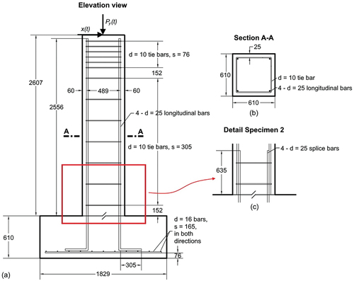
Two full-scale reinforced concrete (RC) specimens representative of pre-1990s bridge column-footing subassemblies were constructed and tested in the iSTAR Laboratory at Portland State University. The specimens were constructed with normal weight concrete and Grade 60 (f_y = 414 MPa) deformed steel bars. The concrete mix was based on a target 28-day nominal concrete cylinder compressive strength of 22.8 MPa. Ready mix concrete was used for the construction with a maximum aggregate size of 19 mm, 100 mm slump, and a water-to-cement ratio of 0.47. A cantilever 610 × 610 mm square cross-section RC column with four 25 mm-diameter continuous longitudinal steel reinforcing bars (rebars) was used for Specimen 1 whereas Specimen 2 had a lap splice located in the plastic hinge zone (see Figure 1). The lap splice length for the dowel bars starting from the column-footing joint was 25d_b (or 635 mm). The transverse reinforcement consisted of 10 mm-diameter square ties with 90-degree hooks at both ends with an extension of 10 times the diameter of the tie bars (or 114 mm). The concrete clear cover from the external face of the tie bars to the face of the column cross section was 25 mm for both of the specimens. The first tie at the bottom of the column region is located 152 mm from the column-footing joint, with subsequent ties spaced at 305 mm. A square spread footing with a single orthogonal layer of 16 mm-diameter rebars spaced at 165 mm located at the bottom was used as the foundation supporting the square column. These two specimens were part of a larger experimental programme sponsored by the Oregon Department of Transportation (ODOT) and were named Test 5 (CR#8) and Test 6 (SS#8) corresponding to Specimen 1 and 2, respectively, and are documented in [3].

Figure 1. Drawings of RC column-footing subassembly test specimens: (a) Elevation view (Specimen 1 and 2), (b) Cross section (Specimen 1 and 2), and (c) lap splice detail Specimen 2. All dimensions in (mm).

2.2. Loading protocol

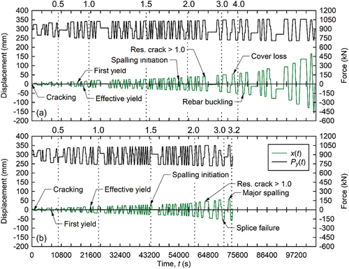
A reverse-cyclic protocol developed to capture the number and amplitude of cycles expected from a subduction earthquake [20] was utilised to assess the seismic performance of the reinforced concrete (RC) column-footing subassembly test specimens. This lateral loading protocol is characterised by a higher number of cycles at the low ductility levels and a lower number of cycles at the higher ductility level. The loading consists of two stages where the first stage includes three nominally elastic cycles, each having peak lateral column top displacements, x(t)_peak corresponding to 0.25δ_i, 0.5δ_i, and 0.75δ_i, followed by one cycle at 1.0δ_i to capture initial damage such as first cracking and the progression of cracks. Here, δ_i is the analytically predicted lateral yield displacement as obtained from monotonic moment curvature analysis of the column cross section. The analytically predicted yield displacement, δ_i for both the specimen was 16.5 mm. The second stage of the protocol consists of inelastic displacement cycles corresponding to increasing levels of ductility, which is defined as the ratio of the displacement to that of the yield displacement:

(1) $\mathit{\mu }=\frac{\mathrm{\Delta }}{{\mathrm{\Delta }}_y}$(1)

Here, Δ is the lateral column top displacement for which the ductility is being calculated and Δ_y is the lateral column displacement resulting in the yield of the column rebars. The subduction protocol targeted a displacement ductility of μ = 8 and a fundamental natural vibration period, T = 0.5 s, which was found to be representative of typical multi-column RC bridge columns [7]. Figures 2(a,b) show the loading protocols for Specimen 1 and 2, respectively. The applied lateral displacement, x(t) following the subduction zone lateral loading protocol as well as the applied varying vertical load, P_y(t) representing the gravity loads on the bridge columns are shown in green and grey, respectively. The varying axial load was implemented to capture the secondary effects on the axial load for multi-column bridge bents. A base axial compression load, P_y = 890 kN was applied initially and the variation in the axial column load was then implemented simultaneously alongside the application of lateral loading protocol. The instances when GPR and UEA measurements were performed are indicated by black vertical dotted lines. The associated numbers represent the corresponding displacement ductility levels, µ. The load application point is shown in Figure 1 with positive and negative values for x(t) being associated with the push and pull directions, respectively. Details of the experimental setup and how the loading protocol was applied to the specimens can be found in [3].

Figure 2. Loading protocol for (a) Specimen 1 and (b) Specimen 2: Applied lateral displacement, x(t) (green lines) and vertical load, Py(t) (grey lines). Vertical black dotted lines with numerical values denote the displacement ductility level, μ.

3. Specimen instrumentation

Several displacement transducers and strain gauges were used to monitor the global and local response of the test specimens. The lateral displacement imposed by the lateral actuator was captured using a load cell and LVDT attached to the actuator. The top displacement of the columns, x(t) was measured with a string potentiometer attached to a fixed reference frame. Applied loads were measured with load cells at each actuator. Strain gauges were used to measure strain in both the longitudinal and dowel bars at critical locations. In addition, three strain gauges were placed at the transverse reinforcement to measure the strain of the tie bars. Details of the instrumentation can be found in [3].

4. Non-destructive testing

An ultrasonic echo array (UEA) instrument with a central pulse frequency of 40 kHz and a time resolution, Δt = 1 μs from Screening Eagle Technologies, Model Proceq Pundit 250 Array, was used to collect data for UEA imaging. The instrument consists of an 8 × 3 array of dry point contact transducers where the three transducers in one row form one independent channel, making it an eight-channel unit. Transducer rows are spaced at 30 mm. Each measurement involves the subsequent transmission of a shear wave pulse into the material channel-by-channel, while the remaining channels record the response. This process produces 28 recorded signals per measurement location. The resulting stress waves travel through the material and are reflected when they reach the boundaries between materials with different acoustic impedances [21]. The selected measurement step (= distance between instrument measurement locations) was 45 mm. A hand-held ground penetrating radar (GPR) instrument was used to collect data along the same scan lines the US data were collected (see Figure 3). The two-channel instrument used was a GSSI, Model StructureScan Mini XT with a central pulse frequency of 2.7 GHz. This unit performs measurements every 2.5 mm, which are triggered automatically by an encoder embedded in the wheels. In GPR, electromagnetic waves are transmitted into a material and are reflected when they reach boundaries between materials with different dielectric properties [14]. More details about these instruments can be found in [15].

Figure 3. Illustrations of test specimen showing GPR/UEA scan lines and sample final reconstructed images: (a) Isometric view from north-east and (b) elevation view of column west face. N = north, S = south, E = east, and W = west. All dimensions in (mm).

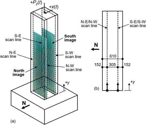
Figure 3 shows the locations of the four scan lines on the east and west faces of the columns. The measurements were taken roughly from the base of the column, but the image reconstruction was started at exactly the base of the column, i.e. at y = 0. The direction of the measurements was bottom to top and was taken when the column was unloaded, i.e. when the lateral load, P_x (t) = 0, at the ductility levels, μ shown in Figure 2.

5. Analysis methodology

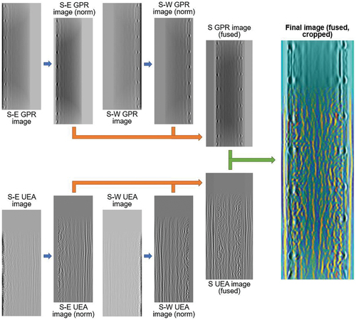
The extended total focusing method (XTFM) [15] was employed to reconstruct the images from both the GPR and the UEA measurements. XTFM is an advanced imaging reconstruction technique that allows for efficient reconstruction of images by considering the entire specimen as a single region instead of stitching and averaging multiple-sub regions. Since both GPR and UEA measurements can be reconstructed using the same XTFM algorithm, the resulting images are compatible for image fusion. This consistency in image reconstruction facilitates a smoother and more accurate integration of the data from both modalities, ultimately providing a clearer and more comprehensive view of interior features.

To have a more complete image of the interior of the specimens, image fusion was employed to include all the information in one frame achieving a comprehensive visualisation [22]. In order to provide an even more complete picture of the columns’ interior, two-sided fusion was implemented to include the information of the west and corresponding east images in one single image. Image fusion allows taking advantage of the strengths of the individual techniques. While GPR is an excellent tool to detect the rebars, US is better at detecting concrete air interfaces, such as a backwall and cracks or the changes in relative reflectivity caused by distributed damage [21]. High reflectivity is an indicator of change in acoustic impedance. Therefore, the information from the two techniques is complementary, supporting a fusion approach. The algorithm used for image fusion is based on a wavelet decomposition [23] where GPR features are shown in greyscale and ultrasonic features are shown in colour. The authors’ previously established pipeline for image reconstruction and fusion was used for this process [15].

Before fusion was performed, standard surface wave removal was applied to both images, and proper normalisation and image registration were applied to make sure the images are in the same pixel range and are aligned horizontally [15]. GPR and UEA from the north and south images were generated using fusion from the corresponding east and west images. The UEA two-sided fused image was colourised using the parula colourmap from MATLAB [24]. The colouring helps to quantify the contribution of each modality in the final fused image. The two-sided GPR and UEA images were then fused together to create a final multimodal fused image. Note that the fusion process was the same for both steps. Each image was decomposed into an approximation coefficient (low pass) and three high detail coefficients (high pass) using a 2D wavelet transform in a recursive fashion four times [15]. The approximations were averaged, and the details maximised. Multi-level wavelet reconstruction was used to obtain the final fused image. Figure 4 illustrates the steps in the image reconstruction and fusion methodology used herein. It can be observed that the GPR and UEA measurements are not available over the same height, which shows in the loss of scatter information from UEA visible in the top region of the final fused image. For consistency, only the region up to y = 1.52 m was thus included in the analysis (see Figures 6,7).

Figure 4. Illustration of image reconstruction and fusion methodology. N = north, S = south, E = east, and W = west.

6. Results and discussion

6.1. Structural performance

Figure 5 shows the lateral load vs. drift ratio plots for the two test specimens. The drift ratio is defined as the ratio of the lateral column top displacement, x(t) to the height of the column. The load-deformation response of Specimen 1, which has continuous longitudinal rebars [see Figure 1 (a)], is characterised by a stable hysteretic response with wide loops at higher displacement ductility levels [Figure 5 (a)]. The peak lateral load recorded in the push direction was 198 kN and the corresponding lateral displacement was 47 mm. In the pull direction, the measured peak load was 169 kN and the displacement was 32 mm. The differences in peak lateral load and corresponding displacement between the push and pull cycles of loading are due to the application of the varying axial load, P_y(t). The push cycle of loading experienced higher compressive axial load compared to the pull cycle. The sequence of damage for Specimen 1 was concrete cracking, yielding of longitudinal reinforcement, initiation of cover spalling, loss of cover concrete, and buckling of longitudinal reinforcement (images and crack maps are reported in [3]). The ultimate displacement capacity of Specimen 1 was 108 mm in the push direction and 139 mm in the pull direction. The corresponding drift ratios at the ultimate displacement capacity were calculated as 4.1% (μ = 5.4) and 5.3% (μ = 7.0), respectively, for the push and pull directions.

Figure 5. Load-drift response of (a) Specimen 1 and (b) Specimen 2.

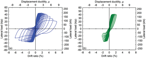
Specimen 2 contains short lap splices of the longitudinal rebars within the plastic hinge zone [see Figure 1(c)] that resulted in lap splice failure. As a result, the load-deformation response of Specimen 2 shows rapid strength degradation in the pull cycle [see Figure 5(b)]. This response can be explained by the short lap splice used in this specimen [see Figure 2(a)]. The peak lateral loads measured in the push and pull directions were 186 kN and 164 kN, respectively. The lateral displacement corresponding to the peak load was 42 mm for both the push and pull directions. Following the peak load, significant strength degradation led to a poor performance of this specimen compared to Specimen 1. The ultimate displacement capacity was 52 mm in the pull direction while in the push direction, the specimen continued to sustain the lateral load carrying capacity. The drift ratio associated with the ultimate displacement capacity was calculated to be 2.0% (μ = 2.9), which is significantly lower than Specimen 1. The sequence of damage is documented with images, and crack maps are reported in [3].

6.2. Qualitative observations

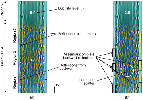
Figure 6 shows sample final fused images from the south side of the column of Specimen 1 for the baseline (μ = 0, prior to loading) and displacement ductility level, μ = 2.0. As can be observed, the images can reveal the backwall as well as reflections from internal cracking and the rebars. Moreover, the backwall portion of the images, which is clear in all baseline states, starts to be shadowed by internal cracking with increasing loading. Indeed, the backwalls are clearly visible in the baseline (= initial, damage free) state, and as loading and therefore damage progresses, the backwall reflection starts to show gaps and a decrease in amplitude. This suggests that the internal cracks are scattering the waves and preventing some energy from reaching the backwall and returning from it. It is also evident that changes in the backwall of the lowest region (i.e. Region 1) are more severe compared to the middle (i.e. Region 2) and especially the top regions (i.e. Region 3). This implies that the bottom regions of the columns experience faster damage progression compared to the upper regions of the column. The images for all selected ductility levels starting from the baseline to failure are provided in Appendix, Figures A1 through A4.

Figure 6. Sample final fused images Specimen 1 (South): (a) Baseline image (μ = 0) and (b) image at ductility level, μ = 2.0. Column width, d = 610 mm. The location and dimensions of the three designated damage regions are shown in Figure 7. Final images for both specimens and additional ductility levels can be found in Appendix, Figures A1 through A4.

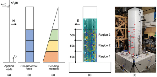
Figure 7 illustrates the applied and resulting internal force distributions in the column, a sample final-fused image with designated damage regions, and a sample photo of a specimen with cracks and designated damage regions highlighted. The damage distribution can be explained by the distribution of the internal forces, namely the bending moment curve, as is illustrated in Figure 7(c). The lowest region of the columns experiences the highest bending moment demand and is thus expected to exhibit the highest level of damage. This is also confirmed by the observed cracks (see [3] for images and crack maps) where we see more cracks in the lower regions of the column.

Figure 7. Illustrations of (a) applied loads, (b) and (c) internal force curves (qualitative), (d) elevation view of specimen north face with sample final reconstructed image and three designated damage regions, and (e) photo of sample specimen during testing with highlighted cracks (red lines) and designated damage regions (dashed black lines). All dimensions in (mm).

6.3. Structural similarity (SSIM) index

From the qualitative observations in Section 6.2, it is possible to observe that the changes in the reconstructed images are not only from the loss of structural information of the image, but also, changes in the luminance and contrast of the images. For example, the missing of the backwall in some parts can be associated with a loss of structural information of the image, while increasing the amplitude of the ultrasonic reflectivity can be related to changes in luminance of the image. The popular SSIM metric [25] from the field of image processing compares three relatively independent terms in two images, namely luminance, contrast, and structure, and hence appears to be an ideal quantitative metric for analysing the fused images. The luminance term, $\mathit{l}$, is related to the intensity of the images, where intensity of an image is defined as the grey-level value assigned to each pixel of a digital image ranging from 0 (= black) to 255 (= white) for an 8-bit image. To compute the luminance term for two images X and Y, we calculate the mean intensities of the images, denoted as ${\mu }_x$ and ${\mu }_y$ respectively. The luminance comparison term is then computed using Equation (2)(2) $\mathit{l}\left(\bar{x},\bar{y}\right)=\frac{2{\mu }_x{\mu }_y+C_1}{{{\mu }_x}^2+{{\mu }_y}^2+C_1}$(2) :

(2) $\mathit{l}\left(\bar{x},\bar{y}\right)=\frac{2{\mu }_x{\mu }_y+C_1}{{{\mu }_x}^2+{{\mu }_y}^2+C_1}$(2)

where $\bar{x}$ and $\bar{y}$ are vectors of interest containing the pixel values of images X and Y, respectively, and $C_1$is a small number to avoid zero division. The contrast term, c, is related to the standard deviation of each image. In other terms, contrast is the variability from the mean value. The contrast term, c is computed using Equation (3)(3) $\mathit{c}\left(\bar{x},\bar{y}\right)=\frac{2{\sigma }_x{\sigma }_y+C_2}{{{\sigma }_y}^2+{{\sigma }_y}^2+C_2}$(3) , as

(3) $\mathit{c}\left(\bar{x},\bar{y}\right)=\frac{2{\sigma }_x{\sigma }_y+C_2}{{{\sigma }_y}^2+{{\sigma }_y}^2+C_2}$(3)

where ${\sigma }_x,{\sigma }_y$ are the standard deviation of the images and $C_2$ is a small number to avoid zero division. The standard deviation of an image describes the variance of pixel intensity values. After subtraction of the luminance, l, from the pixel values, and performing variance normalisation, the structure of the images is compared, which is the correlation coefficient, s, between the images. This correlation coefficient is similar to the metric introduced in [18] and can be calculated using Equation (4)(4) $\mathit{s}\left(\bar{x},\bar{y}\right)=\frac{{\mathit{\sigma }}_{\mathit{xy}}+C_3}{{\sigma }_x{\sigma }_y+C_3}$(4) , as

(4) $\mathit{s}\left(\bar{x},\bar{y}\right)=\frac{{\mathit{\sigma }}_{\mathit{xy}}+C_3}{{\sigma }_x{\sigma }_y+C_3}$(4)

where ${\sigma }_{\mathit{xy}}$ is the cross-covariance of the two images, and $C_3$ is a small number to avoid zero division. Cross-covariance of the two images, ${\sigma }_{\mathit{xy}}$ measures the similarity in the spatial arrangement of pixels between the two images, accounting for the local variations in intensity. At last, the three terms of luminance, contrast, and structure are multiplied together to result in the SSIM metric defined by Equation (5)(5) $\mathit{SSIM}\left(\bar{x},\bar{y}\right)=\left[\mathit{l}\left(\bar{x},\bar{y}\right){]}^{\alpha }.\right[\mathit{c}\left(\bar{x},\bar{y}\right){]}^{\beta }.[\mathit{s}\left(\bar{x},\bar{y}\right){]}^{\gamma }$(5) , as

(5) $\mathit{SSIM}\left(\bar{x},\bar{y}\right)=\left[\mathit{l}\left(\bar{x},\bar{y}\right){]}^{\alpha }.\right[\mathit{c}\left(\bar{x},\bar{y}\right){]}^{\beta }.[\mathit{s}\left(\bar{x},\bar{y}\right){]}^{\gamma }$(5)

where $\mathit{\alpha }$, $\mathit{\beta }$, and $\mathit{\gamma }$ control the relative importance of each measure. If we assign a similar weight of 1 to these variables and assume $C_3=C_2/2$, simplified SSIM values are computed, which is shown in Equation (6)(6) $\mathit{SSIM}\left(\bar{x},\bar{y}\right)=\frac{\left(2{\mu }_x{\mu }_y+C_1\right)\left(2{\sigma }_{\mathit{xy}}+C_2\right)}{({{\mu }_x}^2+{{\mu }_y}^2+C_1)\left({{\sigma }_x}^2+{{\sigma }_y}^2+C_2\right)}$(6) :

(6) $\mathit{SSIM}\left(\bar{x},\bar{y}\right)=\frac{\left(2{\mu }_x{\mu }_y+C_1\right)\left(2{\sigma }_{\mathit{xy}}+C_2\right)}{({{\mu }_x}^2+{{\mu }_y}^2+C_1)\left({{\sigma }_x}^2+{{\sigma }_y}^2+C_2\right)}$(6)

It should be noted that the SSIM value is not computed globally over the entire image, but rather, local SSIM values are computed using an 11 × 11 circular-symmetric Gaussian weighting function with standard deviation of 1.5 samples as suggested by the original article [25]. Given this, the final metric reported for comparison of the images over the entire image is the mean SSIM, which is the average value of SSIM over local windows. We refer to this value as SSIM in the rest of this article for simplicity. This metric is an objective, reference-based index measuring the quality of an image with respect to a baseline image. An SSIM value of 1 means that the two images are identical. Figure 8 shows the SSIM values for the north side and south side of both columns for comparing each loading stage with the corresponding baseline. It can be observed that SSIM values are steadily decreasing over ductility levels, μ = 0.5 to 4.0 (3.2). In addition, the results show a similar trend for both sides and both columns, which demonstrates the reliability of this metric to capture damage progression.

Figure 8. SSIM curves for (a) Specimen 1 and (b) Specimen 2. The dashed horizontal lines at 0.5 and 0.25 are provided for reference (locations arbitrary).

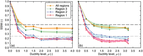
To compare the damage progression along the height of the column, both columns were divided into three regions, each having a height of 508 mm [see Figure 7(d)]. It can be observed that the SSIM values are consistently higher at the base of the column compared to the regions above. This is consistent with the bending moment distribution in the columns, as discussed previously. It can also be seen that the bottom region of Specimen 2 has consistently lower SSIM values than the middle region; however, this is not completely the case for Specimen 1. This difference in the performance of the columns is explored further in the Backwall Analysis section.

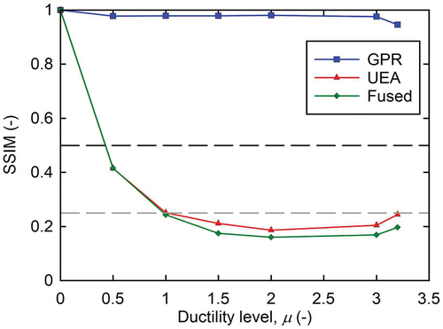
As hypothesised earlier, the internal changes in the fused images are mainly detected by US, and GPR might not be contributing the same level of information. To show the difference in the capabilities of these modalities, the results using only GPR, only UEA, and the fused images were computed. Figure 9 shows the SSIM values across all three regions along column height for the GPR image, the UEA image and the fused image for Specimen 2, north image. It can be observed that the changes are captured by UEA early on, whereas GPR is unable to detect and track the changes. This makes sense since US is sensitive to concrete-air interfaces such cracks, but GPR energy is being reflected mostly from steel rebars. Only at very high levels of damage, i.e. essentially right before failure, does GPR show some sensitivity.

Figure 9. SSIM curves for GPR, UEA, and fused images (for Specimen 2, north image). The dashed horizontal lines at 0.5 and 0.25 are provided for reference (locations arbitrary).

6.4. Backwall analysis

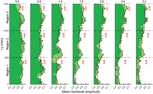
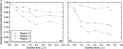
As reported in [18], the shadowing of the backwalls caused by scattering of the US waves can be used as an indicator of damage in a controlled environment. This shadowing effect is also visible in our fused images. However, this effect was not expressed quantitatively in [18]. To quantify this effect, a simple but effective algorithm is presented based on the US images only. In the baseline images [see Figure 6(a) or Appendix, Figures A1 (a) through A4 (a)] it can be seen that the backwall is strongly present, suggesting that there is no damage resulting in wave scattering or blocking. As damage progresses, the backwall amplitude starts to decrease and is sometimes completely undetectable. Figure 10 shows the narrow bands corresponding to the backwall reflections that are tracked across all three regions and throughout the loading process. The centre of a band is the maximum amplitude chosen in a small window where the backwall is present. The width of a band is five pixels, where the maximum amplitude corresponds to its centre. The average of these five pixels is used to calculate backwall intensity at a given location. Figure 11 shows the normalised (to baseline) averaged (over all four backwalls) backwall amplitude values for each region and all ductility levels. From left to right, which corresponds to increasing levels of damage (and increasing ductility levels), for both columns, the mean values of the backwall amplitude are decreasing. This is more visible in Region 1 of the column and less in Regions 2 and 3, which suggests that the bottom regions are more damaged. For Region 3, both columns lose only 8% of the backwall amplitude at the most. This is consistent with the SSIM analysis. Specimen 2 experiences a larger and more sudden loss of amplitude in the backwalls; it suddenly loses backwall amplitude at ductility level, 1.0 of 24%, whereas it is 14% for Specimen 1, and it goes up to 33% whereas it is 21% for Specimen 1. The same holds for Region 2, where Specimen 2 loses 19% of the mean backwall amplitude at ductility level, 1.0, whereas it is 9% for Specimen 1 and it goes to 24% for Specimen 2 and 14% for Specimen 1. This is in line with the findings reported in the Structural Performance section where Specimen 2 exhibits rapid strength degradation due to the presence of the short lap splice compared to Specimen 1.

Figure 10. Illustration of the tracked backwall amplitude bands for Specimen 2, south side. Mean values within the blue and red bands are used in the backwall analysis.

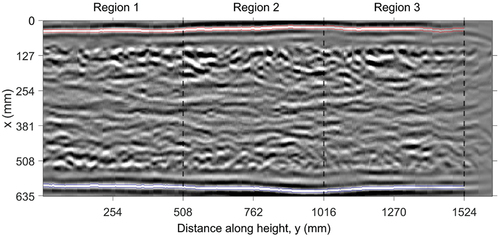
Figure 11. Average normalized backwall amplitude curves per damage region for (a) Specimen 1 and (b) Specimen 2. The values plotted here correspond to the numbers shown in red in Appendix, Figures A5 and A6.

In the Appendix, Figures A5 and A6 show the envelopes of the amplitudes for the four backwalls for Specimens 1 and 2, respectively, as a function of distance along column height, y.

7. Conclusions

In this study, two full-scale reinforced concrete (RC) bridge column-footing subassembly specimens were tested in the laboratory under reverse-cyclic loading and non-destructive testing (NDT) was performed using ground-penetrating radar (GPR) and ultrasonic (US) echo array (UEA) measurements. Images of the interior were reconstructed using the extended total focusing method (XTFM) and image fusion was performed using wavelet decomposition to fuse the images from both modalities and from the east and west scans. The US measurements show the capability of tracking the damage with increasing levels of loading and damage. GPR is unable to capture changes but provides useful information regarding the location of rebars. The results show that internal changes are visible starting from the first measurement after the baseline. In addition, the results show that the base of the column is more damaged compared to the middle and top regions. Visual analyses of backwall amplitude and reflectivity maps are discussed, and the results are quantified using the structural similarity index (SSIM) metric and a backwall amplitude analysis. The SSIM analysis shows that the damage can be tracked from as early as the first measurement after the baseline. The backwall analysis provides a robust way of finding changes in US images and locating damage. Moreover, the backwall analysis agrees with the structural performance observations of the two test specimens. The final fused images show that the bottom region of the column experiences more damage than the middle and top regions and this is confirmed with both SSIM and mean backwall amplitude analysis. Based on the findings of this study and the other studies reviewed in the introduction, we conclude that obtaining a few baseline measurements after construction of a column can be a valuable asset to later examine the condition of a concrete column, for example after an earthquake. GPR measurements are useful for locating metallic features such as rebars and can be used in image fusion to create a more complete image of the interior of a member, but they do not add notable value for capturing damage progression. The introduced SSIM metric represents a valuable tool to detect the changes compared to a baseline. The mean backwall analysis and tracking the backwall is a simple tool that provides useful information in terms of quantifying damage progression, as well as localising damage along a member. While both methods (SSIM and backwall analysis) exhibit sensitivity to degradation, they provide different perspectives on the structure’s condition. The SSIM index captures the overall similarity between images of different loading stages and their corresponding baselines. This method is effective in identifying global damage patterns and trends in a column. In contrast, the backwall analysis directly tracks the loss of backwall amplitude as an indicator of damage. The backwall amplitude decreases with increasing levels of damage, providing a more localised perspective on damage within a column. Overall, the SSIM index offers a broader view of the damage, while the backwall amplitude method provides more localised information about damage progression, thus we suggest using both methods in a complementary manner.

In the future, the use of other modalities and more advanced methods in image reconstruction, especially for the UEA measurements, will be investigated to further quantify the internal changes of the concrete.

Acknowledgments

Full-scale experimental testing was carried out in the infraStructure Testing and Applied Research (iSTAR) Laboratory at Portland State University (PSU) and made possible by the Oregon Department of Transportation (ODOT) through sponsorship of their research project SPR 802 [3]. Additional funding to develop the imaging and image fusion algorithms used in this study was provided by a joint-seed grant from the Oregon Health and Science University (OHSU) and PSU. Research assistants at the iSTAR Laboratory, i.e., Patrick McCoy, Ilya Palnikov, Gregory Norton, Bradley Sharpshair, and Yuhang Wei, assisted with manufacturing, installation, and instrumentation of the test specimens, and their help is greatly appreciated.

Disclosure statement

No potential conflict of interest was reported by the authors.

Data availability statement

The data that support the findings of this study are available from the corresponding author, TS, upon reasonable request.

Additional information

Funding

The work was supported by the Oregon Department of Transportation [SPR 802]; Oregon Health and Science University and Portland State University [Joint-seed grant].

Appendix

Figure A1. Reconstructed images specimen 1, south scan: (a) to (g) correspond to ductility levels, μ = 0.0 (= Baseline) to 4.0, respectively (also shown above region 3). The location and dimensions of the three designated damage regions are shown in Figures 6 and 7.

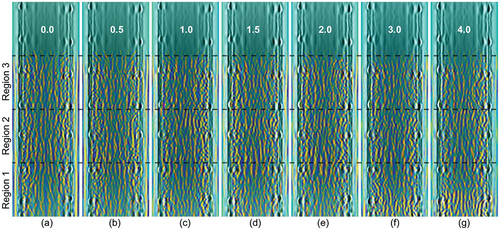
Figure A2. Reconstructed images specimen 1, north scan: (a) to (g) correspond to ductility levels, μ = 0.0 (= Baseline) to 4.0, respectively (also shown above region 3). The location and dimensions of the three designated damage regions are shown in Figures 6 and 7.

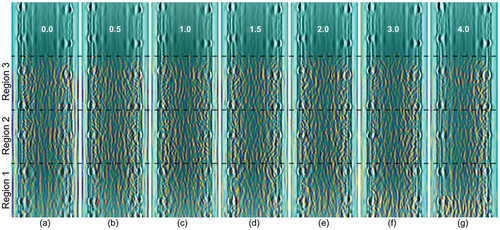
Figure A3. Reconstructed images specimen 2, south scan: (a) to (g) correspond to ductility levels, μ = 0.0 (= Baseline) to 3.2, respectively (also shown above region 3). The location and dimensions of the three designated damage regions are shown in Figures 6 and 7.

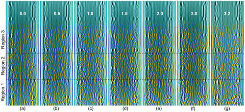
Figure A4. Reconstructed images specimen 2, north scan: (a) to (g) correspond to ductility levels, μ = 0.0 (= Baseline) to 3.2, respectively (also shown above Region 3). The location and dimensions of the three designated damage regions are shown in Figures 6 and 7.

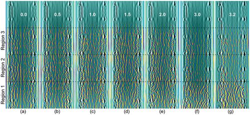
Figure A5. Mean backwall amplitude envelopes from all four images for specimen 1. Red lines and numbers represent the average value across each region. The numbers on top denote the ductility level, μ.

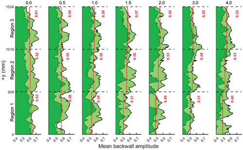
Figure A6. Mean backwall amplitude envelopes from all four images for specimen 2. Red lines and numbers represent the average value across each region. The numbers on top denote the ductility level, μ.

References

- Rojah C. ATC-20-1 field manual: postearthquake safety evaluation of buildings. Applied technology council. Redwood City, CA, USA: Applied Technology Council (ATC); 2005.
- Choi H, Palacios G, Popovics JS, et al. Monitoring damage in concrete columns using ultrasonic tomography. ACI Struct J. 2018;115(2). DOI:10.14359/51701117
- A. K. M. G. Seismic Performance Design Criteria of Existing Bridge Bent Plastic Hinge Region and Rapid Repair Measures of Earthquake Damaged Bridges Considering Future Resilience [ Doctoral Dissertation]. Portland, Oregon: Portland State University; 2022.
- Lehman D, Moehle J, Mahin S, et al. Experimental evaluation of the seismic performance of reinforced concrete bridge columns. J Struct Eng. 2004;130(6):869–879.
- Goodnight JC, Kowalsky MJ, Nau JM. Effect of load history on performance limit states of circular bridge columns. J Bridge Eng. 2013;18(12):1383–1396.
- AL-Hawarneh M, Alam MS. Lateral cyclic response of RC bridge piers made of recycled concrete: experimental study. J Bridge Eng. 2021;26(5):04021018.
- Bazaez R, Dusicka P. Cyclic behavior of reinforced concrete bridge bent retrofitted with buckling restrained braces. Eng Struct. 2016;119:34–48.
- Sasmal S, Voggu S. Nonseismic and seismic designed beam-column joints with rebar end anchors–Behaviour under reverse cyclic loading. J Earthquake Eng. 2021;25(14):2850–2872.
- Holmes C, Drinkwater BW, Wilcox PD. Post-processing of the full matrix of ultrasonic transmit–receive array data for non-destructive evaluation. NDT E Int. 2005;38(8):701–711.
- Moghaddaszadeh M, Adlakha R, Attarzadeh MA, et al. Nonreciprocal elastic wave beaming in dynamic phased arrays. Phys Rev Appl. 2021;16(3):034033.
- Schickert M, Krause M, Müller W. Reconstruction by synthetic aperture focusing technique. Advances And Developments In NDE Techniques For Concrete Structures. 2003;15(3):235.
- Krause M, Mielentz F, Milman B, et al. Ultrasonic imaging of concrete members using an array system. NDT E Int. 2001;34(6):403–408.
- Pashoutani S, Zhu J, Sim C, et al. Multi-sensor data collection and fusion using autoencoders in condition evaluation of concrete bridge decks. J Infrastruct Preserv Resil. 2021;2(1):1–12.
- Clem DJ, Schumacher T, Deshon JP. A consistent approach for processing and interpretation of data from concrete bridge members collected with a hand-held GPR device. Constr Build Mater. 2015;86:140–148.
- Mehdinia S, Schumacher T, Song X, et al. A pipeline for enhanced multimodal 2D imaging of concrete structures. Mater Struct. 2021;54(6):1–16.
- Polimeno MR, Roselli I, Luprano VA, et al. A non-destructive testing methodology for damage assessment of reinforced concrete buildings after seismic events. Eng Struct. 2018;163:122–136.
- Choi H, Popovics JS. NDE application of ultrasonic tomography to a full-scale concrete structure. IEEE Trans Ultrason Ferroelectr Freq Control. 2015;62(6):1076–1085.
- Freeseman K, Khazanovich L, Hoegh K, et al. Nondestructive monitoring of subsurface damage progression in concrete columns damaged by earthquake loading. Eng Struct. 2016;114:148–157.
- Hoegh K, Khazanovich L. Extended synthetic aperture focusing technique for ultrasonic imaging of concrete. NDT E Int. 2015;74:33–42.
- Bazaez R, Dusicka P. Cyclic loading for RC bridge columns considering subduction megathrust earthquakes. J Bridge Eng. 2016;21(5):04016009.
- ACI-American Concrete Institute. 228: 2R-13 report on nondestructive test methods for evaluation of concrete in structures. 2013.
- Kohl C, Krause M, Maierhofer C, et al. 3D-visualization of NDT data using a data fusion technique. Insight-Non-Destructive Test Condition Monit. 2003;45(12):800–804.
- Pajares G, De La Cruz JM. A wavelet-based image fusion tutorial. Pattern Recognition. 2004;37(9):1855–1872.
- MATLAB. Natick, Massachusetts: The MathWorks Inc; 2022a.
- Wang Z, Bovik AC, Sheikh HR, et al. Image quality assessment: from error visibility to structural similarity. IEEE Trans Image Process. 2004;13(4):600–612.