Air quality co-benefits of subnational carbon policies

ABSTRACT

To mitigate climate change, governments ranging from city to multi-national have adopted greenhouse gas (GHG) emissions reduction targets. While the location of GHG reductions does not affect their climate benefits, it can impact human health benefits associated with co-emitted pollutants. Here, an advanced modeling framework is used to explore how subnational level GHG targets influence air pollutant co-benefits from ground level ozone and fine particulate matter. Two carbon policy scenarios are analyzed, each reducing the same total amount of GHG emissions in the Northeast US: an economy-wide Cap and Trade (CAT) program reducing emissions from all sectors of the economy, and a Clean Energy Standard (CES) reducing emissions from the electricity sector only. Results suggest that a regional CES policy will cost about 10 times more than a CAT policy. Despite having the same regional targets in the Northeast, carbon leakage to non-capped regions varies between policies. Consequently, a regional CAT policy will result in national carbon reductions that are over six times greater than the carbon reduced by the CES in 2030. Monetized regional human health benefits of the CAT and CES policies are 844% and 185% of the costs of each policy, respectively. Benefits for both policies are thus estimated to exceed their costs in the Northeast US. The estimated value of human health co-benefits associated with air pollution reductions for the CES scenario is two times that of the CAT scenario.

Implications: In this research, an advanced modeling framework is used to determine the potential impacts of regional carbon policies on air pollution co-benefits associated with ground level ozone and fine particulate matter. Study results show that spatially heterogeneous GHG policies have the potential to create areas of air pollution dis-benefit. It is also shown that monetized human health benefits within the area covered by policy may be larger than the model estimated cost of the policy. These findings are of particular interest both as U.S. states work to develop plans to meet state-level carbon emissions reduction targets set by the EPA through the Clean Power Plan, and in the absence of comprehensive national carbon policy.

Introduction

A variety of jurisdictions at international, national, and subnational scales have set policy targets to reduce emissions of greenhouse gases (GHGs). Major sources of GHGs addressed by these policies are also major sources of conventional air pollutants such as nitrogen oxides (NO_x), sulfur dioxide (SO₂), carbon monoxide (CO), ammonia (NH₃), and volatile organic compounds (VOCs). Therefore, numerous studies have found that policies designed to reduce GHGs will also reduce these other pollutants and their atmospheric products, leading to air quality improvements (Buonocore et al., 2015; Driscoll et al., 2015; Burtraw et al., 2014; Thompson et al., 2014a; West et al., 2013; Muller 2012; Grossman et al., 2011; Nemet et al., 2010; Bell et al., 2008a; Smith and Haigler 2008). Studies also suggest that climate policy would be an effective way to approach an integrated policy that incorporates climate mitigation and air pollution reduction (McCollum et al., 2013; Ravishankara et al., 2012). A key basis for effective policymaking to mitigate both climate and air pollution simultaneously, however, will be to improve understanding about the influence of prospective policies.

Relative to GHGs, the temporal and spatial scales on which conventional pollutant emissions impact humans are short. Whereas emissions of carbon dioxide (CO₂) will change atmospheric chemistry and physics across the globe over tens to thousands of years (Intergovernmental Panel on Climate Change [IPCC], 2013), emissions of co-emitted species such as NO_x and SO₂ are likely to react locally or regionally over a couple of hours or days, often forming secondary pollutants that are harmful to human health. Ozone and fine particulate matter (<2.5 μm; PM_2.5), two pollutants of particular concern (both will be evaluated here), have been linked to negative health impacts, including increased mortality (Pope et al., 2009; Bell et al., 2005). For this reason, whereas GHG emissions reductions in one city could have a positive impact on another continent, any co-benefits associated with reduced air pollution will likely impact the city/region making the reductions, or locations downwind of that city/region.

GHG policies in the European Union and the United States (U.S.) (including the recent U.S. Clean Power Plan) provide flexibility for countries and states to develop unique pathways to individual GHG reduction goals, which may impact co-emitted species differently (U.S. Environmental Protection Agency [EPA], 2014; European Commission [EC], 2010). Thus, as these and other spatially heterogeneous climate policy efforts move forward, assessing local as well as global benefits can inform policy development. Additionally, in the absence of comprehensive national GHG policy in the U.S., regional programs may continue to reduce carbon emissions in a subset of U.S. states, which could change the spatial distribution of co-benefits versus a national policy. Here, we assess the air pollution implications of subnational GHG policy in the U.S., and present policy costs and quantified air pollution-related co-benefits and the potential for dis-benefits.

One challenge associated with a spatially limited carbon cap is the potential for emissions leakage. Studies have found that when emissions caps are placed on a limited area, it is possible for emissions to increase outside of the capped area (Caron et al., 2015; Winchester and Rausch, 2013; Ruth et al., 2008). This “leakage” has the potential to happen for both the target species as well as any co-located emissions. In the case of GHGs, as long as the net change (sum of the total change in both the capped region and the noncapped area) is a decrease in emissions, then the net impact is a benefit to the climate. However, with co-located air pollutants, if the policy results in an increase in emissions anywhere, regardless of the net change, it is likely that some people will be negatively impacted by the policy. In addition, atmospheric chemistry and the transport of pollutants can further shift the burden of pollutants between regions. When considering the health co-benefits of a GHG policy, it is important to evaluate the potential for “leakage” of co-emitted species.

Although many existing air quality co-benefit studies focus examination on electricity sector carbon policies (Buonocore et al., 2015; Driscoll et al., 2015; Burtraw et al., 2014), it is also important to consider the cost-and-benefit trade-offs arising from targeting emissions from the electricity sector compared with a more inclusive economy-wide approach. A previous national co-benefit study found an economy-wide cap-and-trade (CAT) approach to be most cost effective versus policies that cap carbon emissions from only a single sector of the economy, even finding that ancillary benefits of CAT policies can exceed the costs of the policy (Thompson et al., 2014a). Similarly, at a subnational scale, we evaluate how policy design, specifically the sectoral coverage of the GHG emissions cap, will impact costs and benefits associated with the policy, both in the area covered by policy, and outside of that area.

Several studies examine spatially heterogeneous co-benefits of regional climate policy by evaluating unit-level impacts at power plants, finding the largest benefit (and in some cases dis-benefit) to populations living near affected units (Boyce and Pastor, 2013; Aunan et al., 2004). Similarly, Zapata et al. (2013) evaluated state-level GHG policy in California, finding that controlling GHG emissions from five economic sectors produced areas of localized PM_2.5 dis-benefits. Ruth et al. (2008) estimates how the state of Maryland joining the Regional Greenhouse Gas Initiative (RGGI; a market based GHG reduction scheme that includes nine states in the Northeast U.S.) could impact emissions of criteria pollutants both within and outside the state. However, air quality modeling is not included to evaluate human health changes. We build on this literature by considering the potential air quality, health, and related economic impacts of GHG policy scenarios both within and outside of the covered region. We conduct a first analysis at subcountry scale, including full economic, atmospheric chemistry, and health impact modeling, to determine air pollution and human health co-benefits, including potential impacts outside of the area covered.

Here, we present the simulated economic costs and the human health co-benefits of two GHG policy scenarios, applied to 17 states located in the Northeast (NE) U.S. with no constraints on emissions for the rest of the U.S. Our objective is to provide insight into the impacts of subnational (regional) carbon policy. We also show the differences that occur when a single sector of the economy is targeted for carbon emissions reductions versus capping emissions from the entire economy. By discussing results of these regional policies, and comparing our results with those of a previous study evaluating the impacts of identical policies applied nationally, we identify potential feedbacks, the knowledge of which could serve to improve the development of carbon policy with respect to air quality dis-benefits. We aim to inform design of regional carbon policies, as well as state- and federal-level policy design under potential national carbon policies.

Methods

We use a modeling framework developed for the analysis of air quality and human health co-benefits of climate policy that is described in detail in Thompson et al. (2014a). Briefly, this framework links three advanced models to simulate economic and policy responses, air quality, and health outcomes. The United States Regional Energy Policy (USREP) model simulates how the economy will respond to constraints in the form of a carbon policy (Rausch et al., 2010). USREP output is then used to scale emissions inventories for input to the Comprehensive Air quality Model with Extensions (CAMx) for regional photochemical modeling (ENVIRON International Corporation, 2010). CAMx calculates changes in atmospheric pollutants ozone and PM_2.5, which are used as input to the Benefits Mapping and Analysis Program (BenMAP) that calculates human health impacts of air quality changes, and the monetary value of those impacts (Abt Associates Inc., 2013). Previously published analyses using this framework have focused on the evaluation of national-scale carbon policies in the U.S., examining sensitivity to uncertainties (Thompson et al., 2014a) and how health impacts in turn affect the economy (Saari et al., 2015). Here, we implement policy options at a regional scale to evaluate the potential strengths and weaknesses associated with a subnational carbon policy. Each component model is described further below, followed by a description of the policy scenarios applied. Sensitivity to model assumptions are covered in detail in Thompson et al. (2014a). The term “co-benefits” in this paper refers to reductions in ozone and PM_2.5 and the resulting human health benefits that occur as a result of carbon policy.

United States regional energy policy model

The USREP model is a recursive-dynamic computable general equilibrium (CGE) model designed to represent how constraints applied to the economy by climate policy propagate through 17 unique sectors of the economy (Rausch et al., 2010). Four energy commodities are modeled independently, including coal, natural gas, crude oil, and refined oil. Additionally, we identify and model the electricity sector, energy-intensive industry, other industry, private transportation, commercial transportation, agriculture, and service sectors. The following three sectors are each further split by three energy source types (to make nine independently modeled sectors): electric, energy-intensive industry, and other industry are each split into oil, gas, and coal energy sources.

USREP combines the behavioral assumption of rational economic agents with the analysis of equilibrium conditions and represents price-dependent market interactions as well as the origination and spending of income based on microeconomic theory. Profit-maximizing firms produce goods and services using intermediate inputs from other sectors and primary factors of production from households. Utility-maximizing households receive income from government transfers and from their supply to firms of factors of production (labor, capital, land, and resources). USREP is a full employment model. Agents employ full knowledge of historical and present economic conditions in their optimal decisions. Income earned is spent on goods and services or is saved. The government collects tax revenue that is spent on consumption and household transfers.

USREP is based on state-level economic data from the Impact analysis for PLANning (IMPLAN) data set covering all transactions among businesses, households, and government agents for the base year 2006. Energy data from the Energy Information Administration’s State Energy Data System (SEDS) are merged with the economic data to provide physical flows of energy for greenhouse gas accounting. Economic and greenhouse gas data sets in USREP are aggregated to 12 U.S. regions and the 17 commodity groups.

Here, USREP is run to 2030, starting from a 2006 baseline with a 5-yr time step and with policy constraints (described below) starting in 2012. USREP provides changes in production and/or output from each economic sector. Those sectoral changes are then used to scale the corresponding emissions from each sector using the Sparse Matrix Operator Kernel Emissions (SMOKE) emission preprocessing program version 5.1 (Community Modeling and Analysis System [CMAS] Center, 2010). USREP sectors are matched to individual emissions inventory data points using Standard Classification Codes (SCCs) that describe the source activity in detail. For example, SCCs 101001xx, 101002xx, and 101003xx (where x represents any number) represent all external combustion boilers fueled by coal for the purpose of electricity generation (coal-fired power plant). Individual emissions reported from a process at any facility that is assigned one of these codes will be scaled using the ratio from USREP electricity generation by coal: 2030 output versus 2006 output. All SCCs were matched in detail to USREP sectors. This scaling method serves to capture major emissions changes associated with the two policy scenarios, disaggregated by sector. For example, we will capture emissions reductions associated with changes in the transportation sector, e.g., reduced fuel use for either private or commercial vehicles. We neglect within-sector variability: i.e., we will not capture changes associated with fuel switching (gasoline to diesel for example).

The strength of this scaling approach is its ability to incorporate the economy-wide feedbacks captured by USREP. When constraints are applied to any part of the economy (or to multiple parts), there is the potential to change output from sectors and regions both covered and not covered by the policy constraints. By simplifying the scaling process, we clearly identify potential feedbacks resulting from the carbon policy, and these findings may help identify areas of weakness in the development of new policy options. This approach does not account for air quality policy passed after 2010 and therefore does not account for improved air pollution control technologies or additional pollution abatement that might be incentivized through such policy. In the electricity, energy-intensive industry, and other industry sectors, the emissions scaling approach is based on energy use and therefore captures USREP-modeled improvements in energy efficiency as a result of policy. However, our scaling approach effectively assumes constant criteria pollutant emissions factors for all other source sectors. Because we do not include future air quality policy, our 2030 emissions baseline may be high. In previous work, we investigated the sensitivity of benefit results to baseline emissions, finding that benefits decline sublinearly with declining baseline emissions totals (i.e., if baseline emissions are reduced by 25%, the benefits will decline by less than 25%; Thompson et al., 2014a). Other studies have examined the impacts of carbon policy on criteria pollution and associated co-benefits while incorporating air quality policy, but full chemical transport modeling was either used in reduced form as per ton benefits estimates (Akhtar et al., 2013) or not conducted (Loughlin et al., 2011).

We start with a spatially resolved emissions inventory representing 2012 emissions, with hourly detail, developed by the EPA (EPA, 2011a). We calculate policy cost (reported for the year 2030 in 2006 U.S. dollars) as the difference in simulated economic welfare, which includes macroeconomic consumption (capturing market-based activities), and the monetary value of nonworking time (leisure) (Paltsev and Capros, 2013).

Comprehensive air quality model with extensions (CAMx)

The scaled emissions inventories constructed for 2030 (one for each policy scenario plus a “business as usual” case) are then used to drive CAMx version 5.3. CAMx is a photochemical model that simulates the emissions, transport, chemistry, and removal of chemical species in the atmosphere. CAMx is one of the EPA’s recommended regional chemical transport models and is often used by the EPA for air quality analysis (EPA, 2011b, 2007, 2015). Baseline inputs (including meteorological data, emissions inventories, and ancillary files) and model setup parameters for the year-long modeling episode were developed and evaluated by the EPA for use in air quality rulemaking (EPA, 2011a, 2011b; Baker and Dolwick, 2009). Meteorological inputs were developed using the Penn State/National Center for Atmospheric Research Mesoscale Model (MM5), represent conditions as they occurred in 2005 and were held constant for this study (Baker and Dolwick, 2009; Grell et al., 1994). Inventories representing a best approximation of emissions in 2012 were projected from the 2005 base year inventories by the EPA (EPA, 2011a).

Output from CAMx provides concentration data for ozone and PM_2.5, at an hourly time step and user-defined spatial resolution. Ozone and some species that make up total PM_2.5 (including nitrate, sulfate, ammonium, and some organic carbon aerosols) are secondary pollutants, meaning that they are formed in the atmosphere through complex physical and chemical processes and therefore chemical transport models such as CAMx are required in order to estimate the health impacts of policies that affect these two species. Our calculation of total PM_2.5 as presented also includes modeled concentrations of primary species, including black carbon, organic aerosols, and dust. Modeling was conducted in a grid domain covering the continental U.S., with 36 km by 36 km horizontal resolution, found to be appropriate for national-scale health response evaluations (Thompson et al., 2014b).

Benefits mapping and analysis program

CAMx-modeled concentrations of seasonal average daily maximum 8-hr ozone (May through September) and daily average PM_2.5 are input into BenMAP Community Edition version 1.0 to estimate exposure, human health response, and associated monetized benefits to changes in pollution between the “business as usual” (BAU) case and each policy scenario. Modeled changes in ozone and PM_2.5 concentrations and concentration-response functions are combined with census data and county-level mortality incidence rates, both forecast to 2030 (Centers for Disease Control and Prevention [CDC], 2006), to determine changes in health outcomes. No lag time is assumed between exposure and health response, and all monetized benefits are undiscounted.

The mortality concentration-response functions (crfs) applied in this study are peer-reviewed epidemiological studies that estimate increased mortality risk due to changes in ambient concentrations of ozone and PM_2.5 and were presented in the Regulatory Impact Assessment (RIA) conducted by the EPA for the most recent update to the ozone National Ambient Air Quality Standards (EPA, 2015). Morbidity end points include hospital admissions, emergency room visits, school loss days, and acute respiratory symptoms for both pollutants, and acute myocardial infarction (nonfatal heart attacks) and acute bronchitis for PM_2.5. Whereas mortality incidence values are presented individually for each crf, for most morbidity end points, random/fixed-effects pooling is used to combine estimates from individual crfs. Fixed-effects pooling is a method that weights the impact estimated by each study by the inverse of the variance of that study in order to capture the uncertainty associated with all available crfs. Random-effects pooling incorporates both within-study variance and between-study variance. Tables 1 and 2 present, for ozone and PM_2.5, respectively, the crfs and the pooling approach (if applicable) used to estimate benefits in this study. The medians and 95% confidence intervals for incidence values were estimated using 1000 Monte Carlo simulations of the individual or pooled crfs.

Table 1. Incidence values associated with changes to ozone as a result of two regional GHG policies.

			CES		CAT
End Point	Study	Pooling Method	Northeast U.S.	Other U.S.	Northeast U.S.	Other U.S.
Premature mortality—short-term	Smith et al. (2009)	Studies presented individually	39 (19, 58)	−9 (−5, −14)	9 (4, 13)	2 (1, 3)
	Zanobetti and Schwartz (2008)		64 (34, 93)	−16 (−8, −23)	15 (8, 21)	4 (2, 6)
Hospital admissions—respiratory	Katsouyanni et al. (2009)		74 (−17, 165)	−17 (4, −38)	18 (−4, 39)	5 (−1, 10)
Asthma-related emergency department visits	Glad et al. (2012)	Random/fixed-effects pooling	205 (19, 635)	−49 (−154, −5)	21 (2, 62)	12 (1, 36)
	Ito et al. (2007)
	Mar and Koenig (2010)
	Peel et al. (2005)
	Sarnat et al. (2013)
	Wilson et al. (2005)
Asthma exacerbation	Mortimer et al. (2002)	Random/fixed-effects pooling	68971 (−20923, 138957)	−21416 (−43253, 6483)	13905 (−4220, 28032)	4513 (−1369, 9107)
	Schildcrout et al. (2006)
School loss days	Chen et al. (2000)	Random/fixed-effects pooling	50061 (17685, 111203)	−15557 (−34641, −5494)	10083 (3563, 22409)	3280 (1159, 7296)
	Gilliland et al. (2001)
Acute respiratory symptoms	Ostro and Rothschild (1989)		145764 (60137, 230986)	−41550 (−17133, −65879)	28418 (11724, 45034)	9581 (3952, 15185)

Table 2. Incidence values associated with changes to PM_2.5 as a result of two regional GHG policies.

			CES		CAT
End Point	Study	Pooling Method	Northeast U.S.	Other U.S.	Northeast U.S.	Other U.S.
Premature mortality—all-cause	Krewski et al. (2009)	Studies presented individually	4206 (3061, 5341)	863 (628, 1097)	2285 (1663, 2903)	270 (197, 344)
	Lepeule et al. (2012)		9481 (5499, 13422)	1951 (1131, 2765)	5152 (2987, 7295)	613 (355, 869)
	Woodruff et al. (1997)		6 (3, 9)	2 (1, 2)	3 (1, 4)	1 (0, 1)
Nonfatal heart attacks	Peters et al. (2001)	Equal-weights pooling	857 (99, 1862)	185 (21, 401)	491 (56, 1060)	60 (7, 127)
	Pope et al. (2006)
	Sullivan et al. (2005)
	Zanobetti et al. (2009)
	Zanobetti and Schwartz (2006)
Hospital admissions—respiratory	Zanobetti et al. (2009)	Equal-weights pooling	1331 (−241, 2422)	289 (−52, 526)	750 (−136, 1363)	100 (−17, 181)
	Kloog et al. (2012)
Hospital Admissions—chronic lung disease	Moolgavkar (2000)	Random/fixed-effects with others
Hospital admissions—asthma	Babin et al. (2007)	Randon/fixed-effects pooling
	Sheppard (2003)
Hospital admissions—cardiovascular	Zanobetti et al. (2009)	Equal-weights pooling	912 (376, 2094)	183 (88, 408)	495 (198, 1142)	63 (30, 138)
	Peng et al. (2009)
	Peng et al. (2008)
	Bell et al. (2008)
	Moolgavkar (2000)	Sum dependent
Asthma-related emergency department visits	Glad et al. (2012)	Random/fixed-effects pooling	2376 (−412, 4582)	388 (−67, 748)	1395 (−242, 2685)	129 (−23, 247)
	Mar et al. (2010)
	Slaughter et al. (2005)
Acute bronchitis	Dockery et al. (1996)		5281 (−193, 10616)	1134 (−41, 2290)	2873 (−105, 5781)	380 (−14, 769)
Astham exacerbation	Ostro et al. (2001)	Random/fixed-effects pooling	239976 (12715, 1272369)	51322 (2722, 271190)	130294 (6913, 687900)	17101 (911, 99778)
	Mar et al. (2004)
Work loss days	Ostro (1987)		448247 (390536, 505538)	94525 (82370, 106587)	253358 (220795, 285667)	30035 (26198, 33836)
Acute respiratory symptoms	Ostro and Rothschild (1989)		2650745 (2239384, 3058823)	558257 (471792, 643970)	1494595 (1263278, 1723843)	176564 (149497, 203291)
Upper respiratory symptoms	Pope et al. (1991)		97264 (30438, 163588)	20832 (6521, 35027)	52719 (16503, 88640)	6954 (2179, 11682)
Lower respiratory symptoms	Schwartz and Neas (2000)		67239 (32417, 101402)	14318 (6925, 21524)	36197 (17518, 54386)	4657 (2286, 6890)

Note. Values (shown with 95% confidence intervals associated with crf only) are presented for both the policy-covered NE U.S., and all other areas in the U.S. (no policy constraints) for the year 2030.

The dollar value associated with changes in mortality risks is estimated by first using random/fixed-effects pooling to combine results from individual crfs, and then by applying the EPA’s estimate for the Value of a Statistical Life (VSL) based on 26 value-of-life studies (Abt Associates Inc., 2013). The value of morbidity benefits are calculated using an approach that is consistent with the methods in the recent RIA; therefore, we refer readers to this document for more information (EPA, 2015). The morbidity benefits account for less than 6% and 1% of the total value from ozone and PM_2.5 health impacts, respectively. The 95% confidence interval for monetized benefit includes uncertainty associated with individual crfs and with benefits valuation. Both incidence and valuation results represent annual totals for 2030.

Policy scenarios

We implement two subnational carbon policies: a clean energy standard (CES) mandates that a certain fraction of electricity sales has been generated from “clean“ electricity, and a cap-and-trade (CAT) policy covers emissions from all sectors of the economy. The policies are consistent with those applied at national scale by Thompson et al. (2014a). Here, however, policies are applied to 17 states located in the northeastern (NE) U.S., highlighted in gray in Figure 3 (states include Maine, Vermont, New Hampshire, Massachusetts, Connecticut, Rhode Island, New York, Pennsylvania, New Jersey, Delaware, Maryland, West Virginia, Ohio, Indiana, Michigan, Illinois, and Wisconsin). Both policies cover all output from capped sectors that is either produced in the NE U.S., or imported into the NE U.S. This design is equivalent to taxing carbon at the point of consumption, and it has the effect of leveling the playing field for goods produced in that region, versus goods imported from other regions. Therefore, this assumption may overestimate the negative impacts for regions that do not enact policy and who lose market shares from sectors (because any of the goods from these regions that are imported into the region covered by policy are now covered). It will likely underestimate the policy costs of regions that do enact policy, as well as the emissions leakage of both carbon and co-emitted pollutants. All economic modeling simulations start in 2006 and end in 2030, and include economic and population growth. In all simulations, policy constraints start in 2012. We then compare the resulting policy cost and projected air quality co-benefits for the single year of 2030.

By definition, the total year-on-year carbon emissions reductions for both evaluated policy scenarios are equal in the capped 17 states in the NE region of the U.S. Both CAT and CES scenarios lead to a 14% carbon emissions reduction in 2030 and a 4% reduction cumulative from 2012 (when the policies start) to 2030 in the NE states. This is equal to 250 Mt of carbon reduced from the NE states in 2030, and 500 Mt cumulative to 2030. The economic and human health impacts of each policy scenario are compared with a BAU case in which no carbon constraints are applied anywhere in the U.S.

Carbon policy modeling within USREP is based on the development of the CES scenario, where we constrained the model to achieve a certain “clean” (referring to carbon only) electricity fraction target in each modeled year, defined as the ratio of total clean energy electricity generation to total electricity sales. All renewable (wind, solar, hydropower, biopower, and geothermal) and nuclear technologies are considered 100% clean, natural gas with carbon capture and storage (CCS) is considered 95% clean, coal with CCS is considered 90% clean, and gas combined cycle is considered 50% clean. The 500 Mt cumulative reduction is realized by achieving a target of 80% clean energy in 2035 through a linear progression starting at 42% clean energy in 2012. Both the designations of percent clean for each generation type and the clean energy targets are based on the Clean Energy Standard Act of 2012 (U.S. Energy Information Administration [EIA], 2011).

The CAT policy utilizes reductions across all sectors to meet targets, including, but not limited to, the power sector. Additional large reductions in CAT come from industrial sources and transportation, with the largest reductions coming from household consumption. Household consumption represents emissions associated with consuming fossil fuels at the household level and is represented independently from the 17 production sectors previously introduced (an example of consumption is household heating). For the CAT scenario, carbon reductions are set to match those attained by the CES scenario for each model year step. Economic costs for each policy scenario are measured as the annual private consumption loss in 2030 (measured in 2006 U.S. dollars) relative to the BAU case.

Results

We first show the evolution of national total carbon emissions in 5-yr increments (time step of economic model) out to 2030 for each policy scenario and the BAU case. Corresponding changes in total emissions of five air pollutants resulting from both policy scenarios are then presented, followed by impacts on average modeled concentrations of ozone and PM_2.5. These five pollutants (NO_x, CO, SO₂, VOCs, and NH₃) are selected for reporting because they are the major precursors to the formation of ozone and PM_2.5 (however, all emissions from affected sources are scaled in the same way). Finally, changes to incidence rates of human health impacts and the estimated value of those health impacts, resulting from changes in simulated air quality, are presented and the monetized benefit values compared with the costs of each scenario.

Emissions

In the CES scenario, carbon emissions “leakage” is occurring to regions outside of the NE U.S. Although carbon emissions reductions within the 17-state NE region are constant across both regional policy scenarios, the total carbon emissions reduction of the entire U.S. (including regions not capped) is not constant across the scenarios, as shown in Figure 1. The cumulative (2012–2030) total U.S. emissions reductions associated with the regionally implemented CAT scenario are approximately 3 times greater than cumulative emissions reductions associated with the sector specific regionally implemented CES scenario. Nationally in 2030, CAT realizes an annual reduction of 502 Mt, whereas CES reduces only 85 Mt (BAU annual CO₂ emissions are 6230 Mt in 2030). In both scenarios, 250 Mt CO₂ is reduced in the NE U.S. in 2030; therefore, the differences between this number and the emissions reported here, and shown in Figure 1, are due to emissions changes outside of the NE U.S.

Figure 1. Time series of total U.S. carbon emissions from 2010 to 2030 for Business as Usual (no policy; black line), and two subnational carbon cap scenarios applied to the Northeast only: Clean Energy Standard (green dashed line) and Cap and Trade (blue dashed line). Please note range of x-axis.

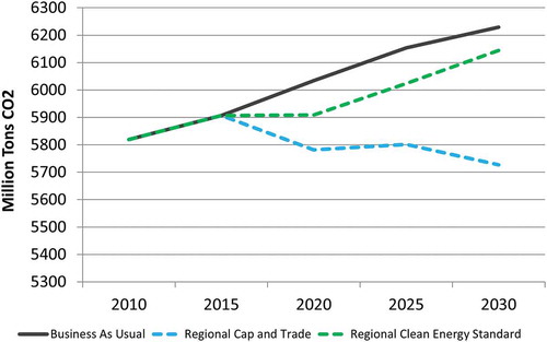
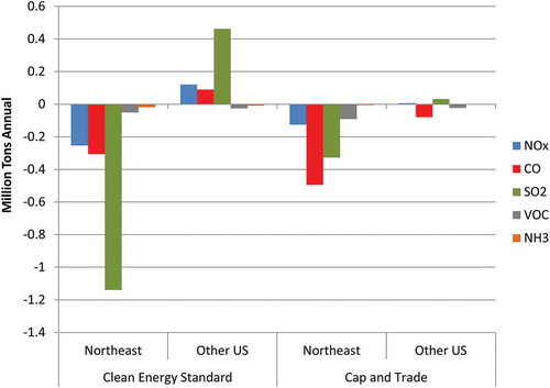
Figure 2. Year 2030 annual change of five common air pollutants (in million tons) due to Clean Energy Standard and Cap and Trade policy scenarios, summed for the Northeast states, and all other states.

Under the CAT scenario, carbon emissions from all goods and services either produced within or imported into the capped region count towards the cap. Under the CES scenario, all emissions from electricity generated for the NE U.S. count towards the cap, but production and sales both within and outside of the capped region can shift to economic sectors not covered. The CES scenario shows greater leakage compared with the CAT scenario because the substitutability between carbon and noncarbon inputs to production and consumption is larger between sectors within a regional economy than between regional economies.

Under CAT, the largest reductions in carbon emissions were made in the NE U.S. in household consumption (which is relatively carbon intensive compared with other sectors), reflecting sizeable adjustments in energy efficiency, fuel switching, and a reduction in demand triggered by the increased costs for fossil-based energy. The next largest reductions were made in the electricity sector, but as costs increased, the CAT scenario allowed the model to draw cheaper cuts from other sectors, including industry, transportation, agriculture, and services.

In contrast to nationwide emissions reductions resulting from the CAT, both carbon and co-emitted pollutant emissions increased in areas outside of the capped region in the CES scenario. CES leads to an increase in coal use in areas outside of the NE (for both the electricity and energy-intensive industry sectors) because more coal is available due to cuts in the NE. This finding does not suggest that new coal-fired power plants are being built in USREP, only that in some areas, existing plants are increasing production because the cost of coal is going down. This is also true for the gas-fired electricity and energy-intensive industry sectors, but to a lesser extent.

Changes in emissions of criteria pollutants, both within and outside of the NE, are driven by the same economic shifts that drive changes to carbon. Figure 2 shows the impact of the carbon policy scenarios, implemented in the NE U.S. only, on emissions of five common air pollutants. Emissions of criteria pollutants decrease in the NE in both scenarios. Similar to the carbon emissions leakage as shown in Figure 1, leakage of emissions of common air pollutants occurs to states outside of the region covered in the CES scenario. In the CES scenario, large decreases in SO₂ emissions are realized in the NE, primarily due to reduction in the output from coal-fired electricity generators. However, SO₂ emissions increase in regions outside of the NE due to increases in electricity generation outside of the capped region. In the CAT scenario, relatively smaller reductions of SO₂, NO_x, and CO are realized mostly from household consumption and electric and industrial coal usage in the NE. Leakage of emissions occurs on a much smaller scale in CAT, with small reductions of every species except NO_x and SO₂ in regions outside of the NE primarily due to small increases in electricity generation outside of the capped region. In reality, criteria pollutant increases out to the future (in the BAU and both scenarios) may be limited in areas with existing emissions controls. Therefore, modeled changes in criteria pollutants due to policy may be overestimated in those areas. However, an important finding from this study is the need for air quality policy to reduce dis-benefit from carbon policy.

Air quality implications

As presented in Figure 3, results of air quality modeling show widespread reductions across the NE U.S. for both ozone and PM_2.5 for every policy scenario. However, areas of increased pollution appear for ozone in both scenarios. Spatial trends in ozone concentration changes are largely driven by corresponding trends in the emissions of precursor species NO_x, CO, and VOCs. An exception occurs over the New York City area in both CAT and CES (and over Chicago in the CES, although this increase is below 0.1 ppb and therefore is not visible in Figure 3) where NO_x emissions reductions lead to local ozone increases. When NO_x emissions are large (as often occurs in population centers with heavy traffic–related emissions), excess NO_x removes ozone, and so the removal of NO_x due to policy increases ozone locally in these locations. PM_2.5 trends shown in Figure 3 are primarily driven by changing SO₂, NO_x, and NH₃ emissions.

Figure 3. Spatial maps showing the modeled changes in ozone (ppb; left column) and PM_2.5 (µg/m³; right column) as a result of three policy scenarios: Clean Energy Standard (top row) and economy-wide Cap and Trade (bottom row). States covered by policy are shown in gray. Ozone results are averaged daily maximum 8 hr from May to September (the “ozone season”), whereas PM_2.5 results are an annual average.

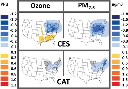
Both ozone and PM_2.5 increase in Texas, the north-central U.S., and the southeastern (SE) U.S. as a result of CES; however, the magnitude of PM_2.5 increases are less than 0.1 µg/m³, which is below the range that would appear in Figure 3.

Health benefits

Tables 1 and 2 present the incidence estimates for the year 2030, with 95% confidence intervals, for both scenarios, for ozone and PM_2.5, respectively. Despite areas of dis-benefit outside of the NE related to increases in ozone, the largest net benefit (including ozone and PM_2.5) to the U.S. as a whole is realized by the CES scenario. Figure 4 shows the monetary benefit of human health changes due to the CES and CAT regional scenarios. Also shown in Figure 4 is the economic cost of each scenario as estimated by USREP. Within the NE region, the value of the human health benefits associated with the CES scenario is likely to outweigh the cost. However, the cost/benefit ratio of the CES scenario in areas outside the capped region is slightly less attractive, due to increases in mortality and morbidity incidences as a result of increasing ozone concentrations.

Figure 4. Economic costs (blue bar) of the regional carbon policies presented with human health co-benefits (black line) associated with each scenario with 95% confidence intervals (gray line) associated with concentration-response functions and valuation. Values are in 2006 U.S. dollars and as a 2030 annual total.

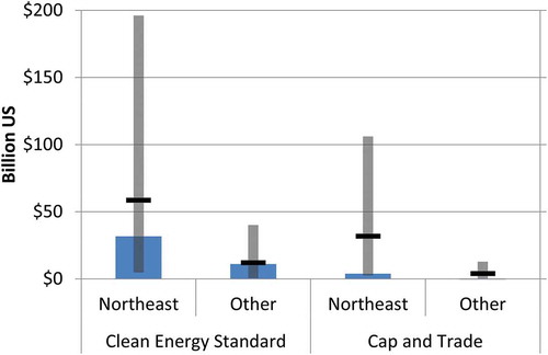
Similar to the assessment of national policies utlizing this modeling framework (Thompson et al., 2014a), we find that the CAT scenario is the cheapest option, with human health co-benefits that are smaller, but similar in scale to those realized/achieved by the CES scenario.

Discussion/policy applications

Our results suggest that, from a co-benefit perspective, regions would benefit most from a cap-and-trade program. This conclusion is based on both the final cost/benefit ratios for each scenario, as well as the occurrence of regions showing ozone dis-benefit due to CES. However, this conclusion is limited by the lack of representation of implementation (administrative) costs in USREP, which may be larger for CAT than other policies. Regardless, clean energy policies are a predominant focus of both national and regional GHG initiatives. The CES results have important implications for GHG policies currently in place at the state level in the U.S. Previous research applied similar CES and CAT policies to the full U.S., showing no areas of PM_2.5 dis-benefit as a result of these two scenarios. Similar to the NE U.S. under the regional carbon policy, the national policy showed a few urban areas with ozone dis-benefit related to decreased NO_x titration as a result of both CAT and CES (Thompson et al., 2014a). Given these comparative findings, regional results presented here could also inform smart design of national policy given the flexibility granted to states by the EPA with regards to meeting targets set by the U.S. Clean Power Plan (CPP). Specifically, the CPP allows for interstate heterogeneity in application that could create areas of air quality dis-benefit. There is also the potential for states to work together under CPP to hit regional carbon targets, which could create a situation similar to what we have evaluated here.

We estimate an average human health co-benefit value of $148/tCO₂ and $80/tCO₂ in the NE U.S. for the CES and CAT scenarios, respectively. We compare these values with those from a previous study we conducted where CES and CAT policies were applied nationally (Thompson et al., 2014a). National co-benefit values of $254/tCO₂ and $140/tCO₂ suggest that sources in the NE U.S. may be cleaner than the national average and therefore health co-benefits not as large. Regional results fall within the range of $2–196/tCO₂ from published literature as reported by Nemet et al. (2010). The values in the Nemet study represent a variety of countries and carbon reduction strategies. In contrast, Butraw et al. (2014) modeled 400 million tCO₂ reduction from the power sector in the U.S. in 2020 and reported benefits of $42.5–55/tCO₂ from human health impacts associated with reduced particulate sulfate concentrations, therefore excluding benefits associated with reduced particulate nitrate and ozone, both from NO_x emissions, and ozone from CO emissions (the latter benefits were included in our analysis). Finally, we estimate 25 and 14 deaths avoided per 1 M tCO₂ avoided (based on pooled mortality results). We compare this with 7.3 deaths avoided per 1 M tCO₂ reduced as reported by Driscoll et al. (2015) in 2020 as a result of a nationwide carbon reduction policy covering the power sector.

In this study, policy costs per tCO₂ reduced in 2030 are $126 and $15 for the CES and CAT scenarios, respectively. When CES and CAT are applied nationally, the policy costs are $255/tCO₂ and $17/tCO₂, respectively, suggesting that the CES scenario may be cheaper to achieve in the NE U.S. versus nationally, and that the cost of the CAT scenario is more consistent in the NE and nationally. We also compare these costs with a range of $12–27/tCO₂ reduced as reported by Burtraw et al. (2014). Burtraw et al. represented costs associated with different strategies of CO₂ reduction from the power sector, but did not model the full economy; therefore, they did not capture potential economy-wide feedbacks as electricity becomes more expensive for all sectors of the economy. In general, the policy costs of imposing carbon policy in the NE U.S. are reflected through increased equilibrium prices for goods and services produced in the NE U.S. Given trade linkages and relatively tightly integrated regional markets, other regions gain market shares at the expense of the NE U.S. Many regions thus show small increases in industry output, including energy-intensive industries and electricity (and their related emissions), as a result of CES.

In our case, the CAT scenario was the least expensive policy option, due to the flexibility inherent in the design. Despite CAT being an order of magnitude cheaper than the CES scenario, human health benefits associated with CAT are not statistically different from the benefits associated with CES. The value of the health benefits associated with CAT were 8 times greater than costs in the NE U.S. This latter finding is supported by previously published studies that suggest that the human health benefits associated with some climate policy options could compensate for some or all of the costs of that policy (Burtraw et al., 2014; Thompson et al., 2014a; IPCC, 2013; Nemet et al., 2010). However, previous research has shown that although policy and economic assumptions do not have a large impact on estimated co-benefit values, they can have a larger impact on policy costs, which could impact the net co-benefit value (Thompson et al., 2014a).

We also find the potential for human health co-benefits outside of the capped area, as a result of the regional CAT, in addition to economic gains to the economy of those areas. Any economic sector importing goods and services into the NE (an area of high population density) has to include CO₂ emissions into the capped area total, thus motivating (or possibly requiring) areas outside of the NE U.S. to make emissions cuts (likely the case with CAT, since all goods are covered). We do not see health disbenefits with CAT because the changes to any one sector are much smaller, thus decreasing the reach of the impact of the policy outside of the NE U.S.

USREP is used here to estimate the impacts, throughout the U.S. economy, of the specifed reduction in emissions of carbon. In practice, these reductions could be reached by either a cap-and-trade approach, or a carbon tax applied to the appropriate sectors of the economy. Our purpose here is to show the potential co-benefits of those realized reductions. We do not attempt to address the merits of different policy designs, including factors that could impact the success of various policy approaches. Our results examine several designs and may inform different policy implementations. However, our analysis does not consider administrative costs or other issues associated with policy implementation.

Although both scenarios lead to aggregate health benefits outside of the capped region, as shown in Figure 3, both scenarios indicate the potential for human health dis-benefits associated with localized increases in ozone. In fact, total health dis-benefits related to ozone were estimated in the CES scenario outside of the region covered (with a projected mortality increase of 9–15 deaths). Previous analyses of ozone and PM_2.5 control policies indicate that human health benefits are dominated by changes in PM_2.5 (Thompson et al., 2014a, 2014b; Fann et al., 2009). As a result, small increases in ozone do not add substantially to the monetary human health burden of a policy relative to small changes in PM_2.5. However, 232 counties in the U.S. are in nonattainment of the 8-hr ozone standard set by the EPA in 2008 (as of 2012; the ozone standard was updated in 2015 and attainment designations have not yet been determined for the new standard [EPA, 2012]), and in those counties, even small increases in ozone would have consequences towards state efforts to bring ozone concentrations back below the standard.

Previous work has shown that overestimation of baseline emissions (emissions of NO_x and SO₂ were 30% and 23% higher, respectively, in 2005 versus 2012, for example) can lead to an overestimation of health benefits (Thompson et al., 2014a). Our BAU case does not include air quality improvements that are likely to occur over time as a result of future policy, and specific future technological improvements. For example, improvements in vehicle efficiency and exhaust emissions out to 2030 as a result of vehicle turnover and policy-driven fuel efficiency improvements are not included, but are not likely to have a major impact on PM_2.5, since that is mostly nonexhaust. Thus, actual co-benefits may be lower than we project here, similar to the limitations of previous work at national scale (Thompson et al., 2014a).

Additional potential benefits to those presented here include the avoided damage from climate change, and potential reductions in air toxics. For example, the benefits estimated here would be in addition to those represented by the Social Cost of Carbon (SCC). The SCC represents monetized marginal damages of CO₂ emissions that include, but are not limited to, reduced agricultural yields, coastal flooding, and increased frequency and severity of weather events (Griffiths et al., 2012).

Overall, this study suggests that an economy-wide subnational carbon policy will lead to regional and national human health co-benefits, and that these co-benefits have the potential to exceed the costs of the carbon policy. Although the same is true for a subnational carbon policy focused on GHG reductions from the electricity sector, we find the potential for areas of air quality dis-benefit with this type of policy, especially with respect to ozone. These increases in ozone, although they have a small impact on the value of aggregate health benefits, would be especially relevant to a region that is not in attainment of national ambient air quality standards for ozone.

Acknowledgment

The authors thank North East States for Coordinated Air Use Management (NESCAUM) for assistance in selection of policy scenarios. The authors also thank the four reviewers for helpful comments that we believe added significant value to this paper.

Funding

The authors acknowledge support from the following: the EPA under the Science to Achieve Results (STAR) program (no. R834279); MIT’s Leading Technology and Policy Initiative; MIT’s Joint Program on the Science and Policy of Global Change and its consortium of industrial and foundation sponsors (see: http://globalchange.mit.edu/sponsors/all); U.S. Department of Energy Office of Science grant DE-FG02-94ER61937; the MIT Energy Initiative Total Energy Fellowship (to R.K.S.); and a MIT Martin Family Society Fellowship (to R.K.S.). Although the research described has been funded in part by the EPA, it has not been subjected to any EPA review and therefore does not necessarily reflect the views of the agency, and no official endorsement should be inferred. The preparation of the manuscript was partially funded by the National Park Service under contract H2370094000. The assumptions, findings, conclusions, judgments, and views presented herein are those of the authors and should not be interpreted as necessarily representing the National Park Service policies.

Additional information

Funding

The authors acknowledge support from the following: the EPA under the Science to Achieve Results (STAR) program (no. R834279); MIT’s Leading Technology and Policy Initiative; MIT’s Joint Program on the Science and Policy of Global Change and its consortium of industrial and foundation sponsors (see: http://globalchange.mit.edu/sponsors/all); U.S. Department of Energy Office of Science grant DE-FG02-94ER61937; the MIT Energy Initiative Total Energy Fellowship (to R.K.S.); and a MIT Martin Family Society Fellowship (to R.K.S.). Although the research described has been funded in part by the EPA, it has not been subjected to any EPA review and therefore does not necessarily reflect the views of the agency, and no official endorsement should be inferred. The preparation of the manuscript was partially funded by the National Park Service under contract H2370094000. The assumptions, findings, conclusions, judgments, and views presented herein are those of the authors and should not be interpreted as necessarily representing the National Park Service policies.

Notes on contributors

Tammy M. Thompson

Tammy M. Thompson is a Research Scientist II at the Cooperative Institute for Research in the Atmosphere (CIRA) at Colorado State University in Fort Collins, CO, USA.

Sebastian Rausch

Sebastian Rausch is an assistant professor at the Department of Management, Technology and Economics at ETH Zurich, Switzerland.

Rebecca K. Saari

Rebecca K. Saari is an assistant professor at the Department of Civil and Environmental Engineering, University of Waterloo in Waterloo, Ontario, Canada.

Noelle E. Selin

Noelle E. Selin is an associate professor at the Massachusetts Institute of Technology in Cambridge, MA, USA.

References

- Abt Associates Inc. 2012. BenMAP, Environmental Benefits Mapping and Analysis Program. User’s Manual, Version 4.0. Research Park Triangle, NC: U.S. Environmental Protection Agency Office of Air Quality Planning and Standards. http://www.epa.gov/airquality/benmap/docs.html ( accessed July 2013).
- Akhtar, F.H., R.W. Pinder, D.H. Loughlin, and D.K. Henze. 2013. GLIMPSE: A rapid decision framework for energy and environmental policy. Environ. Sci. Technol. 47:12011–12019. doi:10.1021/es402283j
- Aunan, K., J. Fang, H. Vennemo, K. Oye, and H.M. Seip. 2004. Co-benefits of climate policy—lessons learned from a study in Shanxi, China. An economic analysis of climate policy: Essays in honour of Andries Nentjes. Energy Policy 32:567–581. doi: 10.1016/S0301-4215(03)00156-3.
- Babin, S.M., H.S. Burkom, R.S. Holtry, N.R. Tabernero, L.D. Stokes, J.O. Davies-Cole, K. DeHaan, and D.H. Lee. 2007. Pediatric patient asthma-related emergency department visits and admissions in Washington, DC, from 2001–2004, and associations with air quality, socio-economic status and age group. Environ. Health 6(1):1. doi:10.1186/1476-069X-6-9.
- Baker, K., and P. Dolwick. 2009. Meteorological Modeling Performance Evaluation for the Annual 2005 Continental U.S. 36-km Domain Simulation. Research Park Triangle, NC: U.S. Environmental Protection Agency Office of Air Quality Planning and Standards. http://www.epa.gov/scram001/meteorology/metgridmodeling/met.2005.36US1.pdf ( accessed April 2015).
- Bell, M.L., D.L. Davis, L.A. Cifuentes, A.J. Krupnick, R.D. Morgenstern, and G.D. Thurston. 2008a. Ancillary human health benefits of improved air quality resulting from climate change mitigation. Environ. Health 7(1):41. doi: 10.1186/1476-069X-7-41.
- Bell, M.L., K. Ebisu, R.D. Peng, J. Walker, J.M. Samet, S.L. Zeger, and F. Dominici. 2008b. Seasonal and regional short-term effects of fine particles on hospital admissions in 202 U.S. counties, 1999–2005. Am. J. Epidemiol. 168(11):1301–1310.
- Bell, M.L., F. Dominici, and J.M. Samet. 2005. A meta-analysis of time-series studies of ozone and mortality with comparison to the national morbidity, mortality, and air pollution study. Epidemiology 16:436–445. doi:10.1097/01.ede.0000165817.40152.85
- Bell, M.L., McDermott A., Zeger S.L., Samet J.M., and F. Dominici. 2004. Ozone and short-term mortality in 95 US urban communities, 1987–2000. JAMA 292:2372–2378. doi: 10.1001/jama.292.19.2372.
- Boyce, J.K., and M. Pastor. 2013. Clearing the air: Incorporating air quality and environmental justice into climate policy. Clim. Change 120:801–814. doi: 10.1007/s10584-013-0832-2.
- Buonocore, J.J., P. Luckow, G. Norris, J.D. Spengler, B. Biewald, J. Fisher, and J.I. Levy. 2015. Health and climate benefits of different energy-efficiency and renewable energy choices. Nat. Clim. Change doi: 10.1038/nclimate2771.
- Burtraw, D., J. Linn, K. Palmer, and A. Paul. 2014. The costs and consequences of Clean Air Act regulation of CO2 from power plants. Am. Econ. Rev. 104:557–562. doi: 10.1257/aer.104.5.557.
- Caron, J., S. Rausch, and N. Winchester. 2015. Leakage from sub-national climate initiatives: The case of California. Energy J. 36:(2). doi:10.5547/ISSN0195-6574-EJ.
- Centers for Disease Control and Prevention. 2006. Morb. Mortal. Wkly Rep. http://wonder.cdc.gov/mmwr/mmwr_reps.asp ( accessed January 2012).
- Chen, L., B.L. Jennison, W. Yang, and S.T. Omaye. 2000. Elementary school absenteeism and air pollution. Inhal. Toxicol. 12:997–1016. doi 10.1080/08958370050164626
- Community Modeling and Analysis System (CMAS) Center. 2010. SMOKE v2.7 User’s Manual. Chapel Hill, NC: Institute for the Environment, The University of North Carolina at Chapel Hill. http://www.smoke-model.org/version2.7/html/( accessed January 2012).
- Dockery, D.W., J. Cunningham, A.I. Damokosh, L.M. Neas, J.D. Spengler, P. Koutrakis, J.H. Ware, M. Raizenne, and F.E. Speizer. 1996. Health effects of acid aerosols on North American children-respiratory symptoms. Environ. Health Perspect. 104:500–505. doi:10.1289/ehp.96104500
- Driscoll, C.T., J.J. Buonocore, J.I. Levy, K.F. Lambert, D. Burtraw, S.B. Reid, H. Fakhraei, and J. Schwartz. 2015. US power plant carbon standards and clean air and health co-benefits. Nat. Clim. Change 5:535–540. doi: 10.1038/nclimate2598.
- ENVIRON International Corporation. 2010. User’s Guide: Comprehensive Air quality Model with Extensions, Version 5.3. Newark, NJ: ENVIRON International Corporation. http://www.camx.com ( accessed January 2012).
- European Commission. 2010. Climate Action: European Union Emissions Trading System. Directorate-General for Climate Action. http://ec.europa.eu/clima/policies/ets/index_en.htm ( accessed December 2014).
- Fann, N., C.M. Fulcher, and B.J. Hubbell. 2009. The influence of location, source, and emission type in estimates of the human health benefits of reducing a ton of air pollution. Air Qual. Atmos. Health 2:169–176. doi: 10.1007/s11869-009-0044-0.
- Fischer, C., and A.K. Fox. 2012. Comparing policies to combat emissions leakage: Border carbon adjustments versus rebates. J. Environ. Econ. Manage. 64:199–216. doi: 10.1016/j.jeem.2012.01.005.
- Gilliland, F.D., K. Berhane, E.B. Rappaport, D.C. Thomas, E. Avol, W.J. Gauderman, et al. 2001. The effects of ambient air pollution on school absenteeism due to respiratory illnesses. Epidemiology 12:43–54. doi:10.1097/00001648-200101000-00009
- Glad, J.A., L.L. Brink, E.O. Talbott, P.C. Lee, X. Xu, M. Saul, and J. Rager. 2012. The relationship of ambient ozone and PM2.5 levels and asthma emergency department visits: Possible influence of gender and ethnicity. Arch. Environ. Occup. Health 62:103–108. doi:10.1080/19338244.2011.598888
- Grell, G., J. Dudhia, and D. Stauffer. 1994. A Description of the Fifth-Generation Penn State/NCAR Mesoscale Model (MM5). NCAR/TN-398+STR. Boulder CO: National Center for Atmospheric Research.
- Griffiths, C., E. Kopits, A. Marten, C. Moore, S. Newbold, and A. Wolverton. 2012. The social cost of carbon: Valuing carbon reductions in policy analysis. In Fiscal Policy to Mitigate Climate Change: A Guide for Policymakers (EPub), eds. R.A. De Mooij, M.M. Keen, and I.W. Parry, Chapter 4. Washington, DC: International Monetary Fund.
- Groosman, B., N.Z. Muller, and E. O’Neill-Toy. 2011. The ancillary benefits from climate policy in the United States. Environ. Resour. Econ. 50:585–603. doi: 10.1007/s10640-011-9483-9.
- Huang, Y., F. Dominici, and M.L. Bell. 2005. Bayesian hierarchical distributed lag models for summer ozone exposure and cardio-respiratory mortality. Environmetrics 16:547–562. doi: 10.1002/env.721.
- Intergovernmental Panel on Climate Change. 2013. IPCC Climate Change 2013: The Physical Science Basis, eds. T.F. Stocker, D. Qin, G.-K. Plattner, M. Tignor, S.K. Allen, J. Boschung, A. Nauels, Y. Xia, V. Bex, and P.M. Midgley. Cambridge, UK: Cambridge University Press.
- Ito, K., S.F. De Leon, and M. Lippmann. 2005. Associations between ozone and daily mortality: Analysis and meta-analysis. Epidemiology 16:446–457. doi: 10.1097/01.ede.0000165821.90114.7f.
- Ito, K., G.D. Thurston, and R.A. Silverman. 2007. Characterization of PM2.5, gaseous pollutants, and meteorological interactions in the context of time-series health effects models. J. Expo. Sci. Environ. Epidemiol. 17(Suppl. 2):S45–S60.
- Katsouyanni, K., J.M. Samet, H.R. Anderson, R. Atkinson, A. Le Tertre, S. Medina, E. Samoli, G. Touloumi, R.T. Burnett, D. Krewski, and T. Ramsay. 2009. Air Pollution and Health: A European and North American Approach (APHENA). Boston, MA: Health Effects Institute, (142), 5–90.
- Kloog, I., B.A. Coull, A. Zanobetti, P.Koutrakis, and J.D. Schwartz. 2012. Acute and chronic effects of particles on hospital admissions in New England. PLoS ONE. 7 (4):1–8.
- Krewski, D., M. Jerrett, R.T. Burnett, R. Ma, E. Hughes, Y. Shi, M.C. Turner, C.A. Pope III, G. Thurston, E.E. Calle, and M.J. Thun. 2009. Extended follow-up and spatial analysis of the American Cancer Society study linking particulate air pollution and mortality. Res. Rep. Health Eff. Inst. 140(5):5–114; discussion 115–136.
- Lepeule, J., F. Laden, D. Dockery, and J. Schwartz. 2012. Chronic exposure to fine particles and mortality: An extended follow-up of the Harvard Six Cities Study from 1974 to 2009. Environ. Health Perspect. 120:965–970. doi: 10.1289/ehp.1104660.
- Levy, J.I., S.M. Chemerynski, and J.A. Sarnat. 2005. Ozone Exposure and mortality: An empiric Bayes metaregression analysis. Epidemiology 16:458–468. doi: 10.1097/01.ede.0000165820.08301.b3.
- Loughlin, D.H., W.G. Benjey, and C.G. Nolte. 2011. ESP v1.0: Methodology for exploring emission impacts of future scenarios in the United States. Geoscientific Model Development 4:287–297. doi:10.5194/gmd-4-287-2011
- Mar, TF, and JQ. Koenig. 2009. Relationship between visits to emergency departments for asthma and ozone exposure in greater Seattle, Washington. Ann Allergy Asthma Immunol. 103:474–479. doi: 10.1016/S1081-1206(10)60263-3.
- Mar, T. F., J. Q. Koenig, and J. Primomo. 2010. Associations between asthma emergency visits and particulate matter sources, including diesel emissions from stationary generators in Tacoma, Washington. Inhal. Toxicol. 22:445–448. doi:10.3109/08958370903575774
- Mar, T. F., T.V. Larson, R.A. Stier, C. Claiborn, and J.Q. Koenig. 2004. An analysis of the association between respiratory symptoms in subjects with asthma and daily air pollution in Spokane, Washington. Inhal. Toxicol. 16:809–815. doi:10.1080/08958370490506646
- McCollum, D.L., V. Krey, K. Riahi, P. Kolp, A. Grubler, M. Makowski, and N. Nakicenovic. 2013. Climate policies can help resolve energy security and air pollution challenges. Clim. Change 119:479–494. doi: 10.1007/s10584-013-0710-y.
- Moolgavkar, S.H. 2000. Air pollution and hospital admissions for diseases of the circulatory system in three U.S. metropolitan areas. J. Air Waste Manage. Assoc. 50:1199–1206. doi:10.1080/10473289.2000.10464162
- Mortimer, K.M., L.M. Neas, D.W. Dockery, S. Redline, and I.B. Tager. 2002. The effect of air pollution on innercity children with asthma. Eur. Respir. J. 19:699–705. doi:10.1183/09031936.02.00247102
- Muller, N.Z. 2012. The design of optimal climate policy with air pollution co-benefits. Resour. Energy Econ. 34:696–722. doi: 10.1016/j.reseneeco.2012.07.002.
- Nemet, G.F., T. Holloway, and P. Meier. 2010. Implications of incorporating air-quality co-benefits into climate change policymaking. Environ. Res. Lett. 5:014007. doi: 10.1088/1748-9326/5/1/014007.
- Ostro, B., M. Lipsett, J. Mann, H. Braxton-Owens, and M. White. 2001. Air pollution and exacerbation of asthma in African-American children in Los Angeles. Epidemiology 12:200–208. doi:10.1097/00001648-200103000-00012
- Ostro, B.D. 1987. Air pollution and morbidity revisited: A specification test. J. Environ. Econ. Manage. 14:87–98. doi:10.1016/0095-0696(87)90008-8
- Ostro, B.D., and S. Rothschild. 1989. Air Pollution and acute respiratory morbidity: An observational study of multiple pollutants. Environ. Res. 50:238–247. doi:10.1016/S0013-9351(89)80004-0
- Paltsev, S., and P. Capros. 2013. Cost concepts for climate change mitigation. Clim. Change Econ. 4(Suppl. 1): 1340003. doi:10.1142/S2010007813400034
- Peel, J.L., P.E. Tolbert, M. Klein, K.B. Metzger, W.D. Flanders, K. Todd, J.A. Mulholland, P.B. Ryan, and H. Frumkin. 2005. Ambient air pollution and respiratory emergency department visits. Epidemiology 16:164–174. doi:10.1097/01.ede.0000152905.42113.db
- Peng, R.D., H.H. Chang, M.L. Bell, A. McDermott, S.L. Zeger, J.M. Samet, and F. Dominici. 2008. Coarse particulate matter air pollution and hospital admissions for cardiovascular and respiratory diseases among Medicare patients. JAMA 299:2172–2179. doi:10.1001/jama.299.18.2172
- Peng, R.D., M.L. Bell, A.S. Geyh, A. McDermott, S.L. Zeger, J.M. Samet, and F. Dominici. 2009. Emergency admissions for cardiovascular and respiratory diseases and the chemical composition of fine particle air pollution. Environ. Health Perspect. 117:957–963. doi:10.1289/ehp.0800185
- Peters, A., D. W. Dockery, J. E. Muller, and M. A. Mittleman. 2001. Increased particulate air pollution and the triggering of myocardial infarction. Circulation 103:2810–2815. doi:10.1161/01.CIR.103.23.2810
- Pope, C.A., D.W. Dockery, J.D. Spengler, and M.E. Raizenne. 1991. Respiratory health and PM10 pollution: A daily time series analysis. Am Rev Respir Dis 144:668–674. doi:10.1164/ajrccm/144.3_Pt_1.668
- Pope, C.A., M. Ezzati, and D.W. Dockery. 2009. Fine-particulate air pollution and life expectancy in the United States. N. Engl. J. Med. 360:376–386. doi: 10.1056/NEJMsa0805646
- Pope, C. A., III, J.B. Muhlestein, H.T. May, D.G. Renlund, J.L. Anderson, and B.D. Horne. 2006. Ischemic heart disease events triggered by short-term exposure to fine particulate air pollution. Circulation 114:2443–2448. doi:10.1161/CIRCULATIONAHA.106.636977
- Rausch, S., G.E. Metcalf, J.M. Reilly, and S. Paltsev. 2010. Distributional implications of alternative U.S. greenhouse gas control measures. B. E. J. Econ. Anal. Policy 10(2). doi: 10.2202/1935-1682.2537.
- Ravishankara, A.R., J.P. Dawson, and D.A. Winner. 2012. New directions: Adapting air quality management to climate change: A must for planning. Atmos. Environ. 50:387–389. doi: 10.1016/j.atmosenv.2011.12.048.
- Ruth, M., S.A. Gabriel, K.L. Palmer, D. Burtraw, A. Paul, Y. Chen, B.F. Hobbs, D. Irani, J. Michael, K.M. Ross, R. Conklin, and J. Miller. 2008. Economic and energy impacts from participation in the regional greenhouse gas initiative: A case study of the State of Maryland. Energy Policy 36:2279–2289. doi: 10.1016/j.enpol.2008.03.012.
- Saari, R.K., N.E. Selin, S. Rausch, and T.M. Thompson. 2015. A self-consistent method to assess air quality co-benefits from U.S. climate policies. J. Air Waste Manage. Assoc. 65:74–89. doi: 10.1080/10962247.2014.959139.
- Sarnat, J.A., S.E. Sarnat, W.D. Flanders, H.H. Chang, J. Mulholland, L. Baxter, and H. Ozkaynak. 2013. Spatiotemporally resolved air exchange rate as a modifier of acute air pollution-related morbidity in Atlanta. J. Expo. Sci. Environ. Epidemiol. 23(6):606–615. doi: 10.1038/jes.2013.32.
- Schildcrout, J.S., L. Sheppard, T. Lumley, J.C. Slaughter, J.Q. Koenig, and G.G. Shapiro. 2006. Ambient air pollution and asthma exacerbations in children: An eight-city analysis. Am. J. Epidemiol. 164:505–517. doi:10.1093/aje/kwj225
- Schwartz, J. 2005. How sensitive is the association between ozone and daily deaths to control for temperature? Am. J. Respir. Crit. Care Med. 171:627–631. doi: 10.1164/rccm.200407-933OC.
- Schwartz, J., and L.M. Neas. 2000. Fine particles are more strongly associated than coarse particles with acute respiratory health effects in schoolchildren. Epidemiology 11:6–10. doi:10.1097/00001648-200001000-00004
- Sheppard, L. 2003. Ambient air pollution and nonelderly asthma hospital admissions in Seattle, Washington, 1987–1994. In Revised Analyses of Time-Series Studies of Air Pollution and Health, 227–230. Special Report. Boston, MA: Health Effects Institute.
- Slaughter, J.C., E. Kim, L. Sheppard, J.H. Sullivan, T.V. Larson, and C. Claiborn. 2005. Association between particulate matter and emergency room visits, hospital admissions and mortality in Spokane, Washington. J. Expo. Anal. Environ. Epidemiol. 15(2):153–159. doi:10.1038/sj.jea.7500382
- Smith, K.R., and E. Haigler. 2008. Co-benefits of climate mitigation and health protection in energy systems: Scoping methods. Annu. Rev. Public Health 29:11–25. doi: 10.1146/annurev.publhealth.29.020907.090759.
- Smith, R.L., B. Xu, and P. Switzer. 2009. Reassessing the relationship between ozone and short- term mortality in U.S. urban communities. Inhal. Toxicol. 21:37–61. doi:10.1080/08958370903161612
- Sullivan, J., L. Sheppard, A. Schreuder, N. Ishikawa, D. Siscovick, and J. Kaufman. 2005. Relation between short-term fine-particulate matter exposure and onset of myocardial infarction. Epidemiology 16:41–48. doi:10.1097/01.ede.0000147116.34813.56
- Thompson, T.M., S. Rausch, R.K. Saari, and N.E. Selin. 2014a. A systems approach to evaluating the air quality co-benefits of US carbon policies. Nat. Clim. Change 4:917–923. doi: 10.1038/nclimate2342.
- Thompson, T.M., R.K. Saari, and N.E. Selin. 2014b. Air quality resolution for health impact assessment: Influence of regional characteristics. Atmos. Chem. Phys. 14:969–978. doi: 10.5194/acp-14-969-2014.
- U.S. Energy Information Administration. 2011. Analysis of impacts of a clean energy standard as requested by Chairman Bingaman. http://www.eia.gov/analysis/requests/ces_bingaman/ ( accessed May 2016).
- U.S. Environmental Protection Agency. 2007. Guidance on the Use of Models and Other Analyses for Demonstrating Attainment of Air Quality Goals for Ozone, PM2.5, and Regional Haze. Office of Air Quality Planning and Standards. http://www.epa.gov/scram001/guidance/guide/final-03-pm-rh-guidance.pdf (accessed May 2016).
- U.S. Environmental Protection Agency. 2011a. Emissions Inventory Final Rule. Office of Air Quality Planning and Standards. http://www.epa.gov/airtransport/CSAPR/pdfs/EmissionsInventory.pdf ( accessed January 2013).
- U.S. Environmental Protection Agency. 2011b. Air Quality Modeling Final Rule Technical Support Document. Office of Air Quality Planning and Standards. http://www.epa.gov/airtransport/pdfs/AQModeling.pdf ( accessed January 2013).
- U.S. Environmental Protection Agency. 2011c. Regulatory Impact Analysis for the Federal Implementation Plans to Reduce Interstate Transport of Fine Particulate Matter and Ozone in 27 States. Office of Air and Radiation. http://www.epa.gov/airtransport/pdfs/FinalRIA.pdf ( accessed January 2013).
- U.S. Environmental Protection Agency. 2012. Area Designations for 2008 Ground-Level Ozone Standards. Office of Air and Radiation. http://www.epa.gov/airquality/ozonepollution/designations/2008standards/index.htm, ( accessed November 2014).
- U.S. Environmental Protection Agency. 2014. Clean Power Plan Proposed Rule. http://www2.epa.gov/carbon-pollution-standards/clean-power-plan-proposed-rule ( accessed December 2014).
- U.S. Environmental Protection Agency. 2015. Technical Support Document (TSD), Preparation of Emissions Inventories for the Version 6.2, 2011 Emissions Modeling Platform. Office of Air Quality Planning and Standards, Air Quality Assessment Division. http://www3.epa.gov/ttn/chief/emch/index.html#2011 ( accessed January 2016).
- West, J.J., S.J. Smith, R.A. Silva, V. Naik, Y. Zhang, Z. Adelman, M.M. Fry, S. Anenberg, L.W. Horowitz, and J.-F. Lamarque. 2013. Co-benefits of mitigating global greenhouse gas emissions for future air quality and human health. Nat. Clim. Change 3:885–889. doi: 10.1038/nclimate2009.
- Wilson, A.M., C.P. Wake, T. Kelly, T., and J.C. Salloway. 2005. Air pollution and weather, and respiratory emergency room visits in two northern New England cities: An ecological time-series study. Environ. Res. 97:312–321. doi:10.1016/j.envres.2004.07.010
- Winchester, N., and S. Rausch. 2013. A numerical investigation of the potential for negative emissions leakage. Am. Econ. Rev. 103:320–325. doi: 10.1257/aer.103.3.320.
- Woodruff, T.J., J. Grillo, and K.C. Schoendorf. 1997. The relationship between selected of postneonatal infant mortality and particulate air pollution in the United States. Environ. Health Perspect. 105:608–612. doi:10.1289/ehp.97105608
- Zanobetti, A., M. Franklin and J. Schwartz. 2009. Fine particulate air pollution and its components in association with cause-specific emergency admissions. Environmental Health 8:58–60.
- Zanobetti A., and J. Schwartz. 2006. Air pollution and emergency admissions in Boston, MA. J. Epidemiol. Community Health 60:890–895. doi:10.1136/jech.2005.039834
- Zanobetti, A, and J. Schwartz. 2008. Mortality displacement in the association of ozone with mortality: An analysis of 48 cities in the United States. Am. J. Respir. Crit. Care Med. 177:184–189. doi:10.1164/rccm.200706-823OC
- Zapata, C., N. Muller, and M.J. Kleeman. 2013. PM2.5 co-benefits of climate change legislation part 1: California’s AB 32. Clim. Change 117:377–397. doi: 10.1007/s10584-012-0545-y.