Modeling vehicle interior noise exposure dose on freeways: Considering weaving segment designs and engine operation

ABSTRACT

Vehicle interior noise functions at the dominant frequencies of 500 Hz below and around 800 Hz, which fall into the bands that may impair hearing. Recent studies demonstrated that freeway commuters are chronically exposed to vehicle interior noise, bearing the risk of hearing impairment. The interior noise evaluation process is mostly conducted in a laboratory environment. The test results and the developed noise models may underestimate or ignore the noise effects from dynamic traffic and road conditions and configuration. However, the interior noise is highly associated with vehicle maneuvering. The vehicle maneuvering on a freeway weaving segment is more complex because of its nature of conflicting areas. This research is intended to explore the risk of the interior noise exposure on freeway weaving segments for freeway commuters and to improve the interior noise estimation by constructing a decision tree learning–based noise exposure dose (NED) model, considering weaving segment designs and engine operation. On-road driving tests were conducted on 12 subjects on State Highway 288 in Houston, Texas. On-board Diagnosis (OBD) II, a smartphone-based roughness app, and a digital sound meter were used to collect vehicle maneuvering and engine information, International Roughness Index, and interior noise levels, respectively. Eleven variables were obtainable from the driving tests, including the length and type of a weaving segment, serving as predictors. The importance of the predictors was estimated by their out-of-bag–permuted predictor delta errors. The hazardous exposure level of the interior noise on weaving segments was quantified to hazard quotient, NED, and daily noise exposure level, respectively. Results showed that the risk of hearing impairment on freeway is acceptable; the interior noise level is the most sensitive to the pavement roughness and is subject to freeway configuration and traffic conditions. The constructed NED model shows high predictive power (R = 0.93, normalized root-mean-square error [NRMSE] < 6.7%).

Implications: Vehicle interior noise is usually ignored in the public, and its modeling and evaluation are generally conducted in a laboratory environment, regardless of the interior noise effects from dynamic traffic, road conditions, and road configuration. This study quantified the interior exposure dose on freeway weaving segments, which provides freeway commuters with a sense of interior noise exposure risk. In addition, a bagged decision tree–based interior noise exposure dose model was constructed, considering vehicle maneuvering, vehicle engine operational information, pavement roughness, and weaving segment configuration. The constructed model could significantly improve the interior noise estimation for road engineers and vehicle manufactures.

Introduction

Sound originates as vibrations in the air causing pressure disturbances that hit our eardrums (Tingwall, 2015). The dominant frequency that a sound wave oscillates per second is the distinct pitch for our ears. The vibrations measured from a vehicle that are unintentionally generated are considered vehicle interior noise for drivers, which is usually a result of the vibrations from engine operation, vehicle maneuvering, such as speed, acceleration, and braking, and other operational circumstances, such as pavement materials and roughness, wind force, tired materials, weather, traffic flow, ambient vehicles, etc. (Crocker, 2007; Hibbs and Larson 1996; Li et al., 2016a; Liang et al., 2012; Qiao et al., 2016; Sandberg and Ejsmont, 2002; Li et al., 2016b). Previous studies have proven that the vehicle interior noise on freeways could be up to 93 dB(A) and a heavy-duty truck passing can emit 90 dB(A) at 15.24 m (50 ft) distance (Klein, 2003). When driving speed is greater than 70 km/hr, the interior noise could exceed the public health and welfare safe limit 75 dB(A) (U.S. Environmental Protection Agency [EPA], 1974). However, the road configuration that requires various vehicle maneuvering, particularly freeway weaving segments (Liu et al., 2017; You et al., 2016), has been seldom investigated for its impacts on the interior vehicle noise. Likewise, the engine operational information attributed to the complex weaving maneuvering is generally excluded in the interior noise modeling.

In practice, an engine is dynamically operated, thereby generating interior noise at varied levels, vibrations of which derive from cylinders for combustion and the corresponding pressure waves in the intake and exhaust systems. The vibrations are very sensitive to the rotational speed of an engine, namely, revolutions per minutes (RPM), and engine loads (DriverSide, 2016). The RPM is a function of the design of the engine and the power supply and is regulated by a signal from two accelerator pedal sensors, D and E, which detect the degree of accelerator pedal position in percentage for determining the amount of torque for a desired vehicle speed. Thus, the RPM is determinative for the vehicle’s operational modes. The engine load is a measure of power output or fuel consumption to directly support the vehicle’s dynamic operational modes. The engine load is represented by calculated engine load (cLoad) and absolute engine load (aLoad). Whereas the cLoad indicates the percentage of peak available torque and is linearly correlated with an engine vacuum, the aLoad is a normalized value of air mass per intake stroke in percentage (SAE International, 1991). Apparently, these multiple and interactive variables raise the difficulties in the interior noise controls and modeling.

Additionally, most noise pollution controls are concerned with specific sources, particularly work places, rather than typical cumulative daily exposure (EPA, 1974). For example, the occupational noise at work places is regulated by the Occupational Safety and Health Administration (OSHA) to the limits of 85 and 90 dB(A) for 8-hr exposure (OSHA, 1999). Nevertheless, Flamme et al. (2012) reported that a large portion of the general population is daily exposed to the noise level that could lead to chronic adverse effects on hearing, and most of them do not even engage in a noisy job. This implies that we may have been unconsciously exposing to the noise levels that are not conventionally considered as hazard. Moreover, a recent study (Li et al., 2017) found that freeway commuters are chronically exposed to the vehicle interior noise at the level between 75 and 85 dB(A), bearing the risk of hearing impairment. The interior noise functions at the dominant frequencies of 500 Hz below and around 800 Hz, which fall into the frequency bands that may impair hearing, such as inability to hear and understand speech (Park et al., 2003).

Although vehicle manufactures have been making great efforts in the interior noise controls, their attention is limited to mobility and engineering perspectives, such as innovation of vehicle technologies, and tire quality. A number of automotive interior noise models have been developed, such as low-frequency finite element (FE) models, airborne statistical energy analysis (SEA) models, structure-borne SEA models, etc. (Kim and Kim, 2000; Park et al., 2003; Shorter, 2008). Nevertheless, the interior noise tests and models are usually conducted in a laboratory environment, regardless of dynamic traffic, road conditions and configuration, and engine operational information. With respect to these multiple variables, feature selection technique could be applied to identify important variables for the response of the interior noise levels. Besides, nonparametric and nonlinear machine learning algorithms, such as decision tree, could be adopted to learn from the complex data without relying on rules-based programming. Instead, decision tree provides a simple framework for prediction, which is more flexible than parametric models (Frigola-Alcade, 2015; Srivastava, 2015). Although overfitting may be more likely with these machine learning algorithms, it could be addressed by pruning a tree after it has learned to remove some of the details from the training process, such as penalty method, holdout, and k-fold cross-validation method, and ensembles (Brownlee, 2016).

This research is proposed to explore the risk of the vehicle interior noise exposure on weaving segments for freeway commuters and to improve the interior noise estimation by constructing a bagged decision tree (BDT)-based interior noise exposure dose (NED) model, taking into account vehicle maneuvering, engine operation, pavement roughness, and weaving configuration.

Methodology

Noise exposure measures

In this study, vehicle interior noise was measured by normalized noise equivalent exposure doses (NEDs) in percentage form, indicating a saturated level of a marginal noise safe limit, and normalized noise levels () over 8 hr of exposure in decibel form. A total equivalent exposure time factor (EETF) in sec/km and the distribution per weaving trip were estimated to quantify the possible hazardous noise exposure (greater than thresholds) on freeways. The occupational noise limit 8-hr 85 dB(A) was adopted as a threshold to estimate the NED and . In other words, when drivers are exposed to 85 dB(A) for 8 hr in a day, the NED reaches the saturated level 100% and the is 85 dB(A). Besides, the noise limits 8-hr 85 dB(A) and 8-hr 90 dB(A) were applied to the EETF calculation as thresholds.

Noise equivalent exposure dose

Each sound record (L) is A-weighted sound level linearly energy averaged over a certain duration in decibel per T hr. To evaluate the hazardous level, all the sound records are normalized to an equivalent exposure dose (NED) in percentage, indicating the saturated level of an 8-hr 85 dB(A) exposure, using eq 1 (NoiseMeters Inc., 2017).

(1)

where NED is the normalized noise equivalent exposure dose for the threshold 8-hr 85 dB(A) exposure (%); T is the sampling time (hr) of each measurement, it is 1/7200 hr or 0.5 sec in this study; and L is the real measured sample of A-weighted sound level linearly energy averaged over T hr.

Equivalent daily noise exposure level

is A-weighted sound level linearly energy averaged over 8 hr in decibel for a day. The is an equivalent noise level for 8-hr 85 dB(A) exposure, as the real measured sample is the noise level energy averaged over T hr. When the is equal to or greater than 85 dB(A), the noise exposure is saturated for a day. Further excessive exposure may bring about a higher hazard of developing adverse health effects. Equation 2 depicts the conversion from the NED to the for each sample (NoiseMeters Inc., 2017).

(2)

Total equivalent exposure time factor

EETF is the average exposure time to the noise levels that are equal to or greater than thresholds, in seconds per kilometer driving distance (sec/km). All noise records that are greater than the threshold are converted to a marginal noise exposure time in seconds, based on 3-dB exchange rule, which are summed to a total equivalent exposure duration and then divided by the total distance traveled during the exposure period, expressed by eq 3 (Li et al., 2017).

(3)

where L_threshold is 85 or 90 dB(A) exposure daily for 8 hr; n is the total number of observations/samples that are greater than the L_threshold; L_i is the ith real measured sample, the observed noise level of which is greater than the L_threshold; and d_traveled is the total travel distance in km during the exposure period.

Hazard quotient of interior noise exposure

According to EPA (2011), hazard quotient (HQ) is the ratio of the potential exposure to the substance and the level at which no adverse effects are expected. The HQ less than or equal to 1 indicates that adverse effects are not likely to occur, and the exposure is considered as negligible hazard. If the HQ is greater than 1, the HQ presents whether and by how much an exposure concentration exceeds the reference concentration. The adverse effects do not necessarily take place. The HQ is not a statistical probability of harm occurring. Instead, it represents the potential of developing adverse effects.

The HQ was adopted to estimate the potential of developing adverse health effects resulting from daily exposure to interior noise. As the threshold of noise exposure is a level of 8-hr exposure, each real measured interior noise level was normalized to 8-hr exposure level () and divided by the threshold, as illustrated in eq 4.

(4)

The HQ values that are less than or equal to 1 are considered indicative of acceptable hazard. Otherwise, the potential of developing adverse effects increases.

Bagged decision tree–based interior noise exposure dose model

Interior noise exposure dose model

Vehicle interior noise levels are a result of multiple and interactive variables from engine operation, vehicle maneuvering, and other operational circumstances. The relationship between these variables and NED could be nonparametric and nonlinear. Decision trees are nonparametric and highly robust. Meanwhile, The decision tree itself presents several notable advantages over other mining methods, including simple to understand and interpret, little data required for preparation, robustness with missing data, etc. (Chen, 2009). However, tree-based methods typically are not competitive with the best supervised learning approaches, in terms of prediction accuracy for overfitting. To overcome the overfitting, BDT algorithm, adding bootstrap aggregating method to the decision tree model, was chosen to construct an NED model in this study.

The BDT is an ensemble method to aggregate the predictions from multiple grown decision trees to make more accurate predictions than any individual decision tree model. The decision trees grow by a bootstrap method, in which a number of random subsamples of original and single training data set are generated with replacement. Each bootstrap sample is taken from two-thirds (63%) of unique observations in the original training data set to train a predictor (Breiman, 1996a). One-third (37%) of the observations that is not included in the bootstrapping is the out-of-bag samples or OOB (Breiman, 1996b). The predicted NED, , is the average predicted NED from each model.

A consensus prediction is the weighted average of all the predictions from the bootstrapped data sets of the selected ensembles, the algorithm of which is described in eq 5 (Breiman, 1996b).

(5)

where is the modeled NED for an entire ensemble; is the modeled NED from tree m in the ensemble; S is the set of indices of selected trees that compose the prediction; is the weight of tree m; and equals 1 if m is in the set S, and 0 otherwise.

The OOB observations are used to estimate the modeling performance. The trained ensemble is applied to the subset of OOB observations in each tree to predict the response NED. For a single tree, the difference between the OOB-predicted responses and the observed responses is the OOB error. The OOB error of the trained ensemble is the average of all OOB errors in all trees. The average OOB error is an unbiased estimator of the true ensemble error (Breiman et al., 1984).

Predictor importance

All relevant available variables from the driving tests are regarded as predictors for the NED model. The importance of the predictor is indicated by the OOB-permuted predictor delta errors in the structured bagged decision trees. The important predictors are deemed as independent variables for the NED model. This is to measure the increase in prediction error if the variable values are permuted across the out-of-bag observation, which is computed for every tree. The representative importance for the variable is an average of the prediction errors from the entire ensemble divided by the standard deviation over the entire ensemble.

Modeling accuracy measurement

The Pearson correlation coefficient and normalized root-mean-square error (NRMSE) are adopted to evaluate the prediction accuracy by the BDT-based NED model.

The Pearson correlation coefficient is a measure of the linear dependence correlation relationship between two data sets, which is signified by R in its calculation shown in eq 5 (Pearson, 1895).

(5)

where n is the total number of in-vehicle noise samples; is the ith sample of a data set x, which could be modeled NED or observed NED; is the ith sample of another data set y, which could be observed NED or modeled NED, respectively; is an average of the data set ; and is an average of the data set .

The R value ranges from −1 to +1 for negative and positive linear correlations, respectively. When R is close to 0, the two data sets are not linearly correlated.

The NRMSE represents the sample standard deviation of the difference between predicted values and observed values; the lower the NRMSE, the higher the accuracy of the NED model. Equation 6 shows that calculation of the NRMSE.

(6)

where is the modeled NED value for the ith observation; is the ith observed NED value; n is the total number of observations in data set; are the maximum observed values in the data set; and are the minimum observed values in the data set.

Data collection and processing

An on-road driving test was conducted on 12 subjects, who held a valid Texas driver license, on the State Highway (SH) 288 in Houston, Texas, during peak and nonpeak hours of a sunny weekday in May 2016. Each subject drove the same vehicle, 2015 Nissan Sentra, from the entrance of Southmore Street on SH 288 to the exit of Shadow Creek Parkway towards the direction to the City of Pearland, then turned back to the exit of Southmore Street. In between, subjects were required to get off the highway at the exit of Holcombe Boulevard, Reed Road, West Orem Drive, Bellfort Street, and Yellowstone Boulevard, and get on at the next entrance, respectively. The test route is about 35 km (22 miles) in length. On the test route, subjects drove through six segments in three different types with different lengths, including Types A, B, and C. The type of weaving segments is defined by the number of minimum lane changes required for weaving (Highway Capacity Manual [HCM 2000]; Transportation Research Board, 2000). Figure 1 illustrates the configuration of the three types of waving segments.

Figure 1. Weaving segment configuration (a) Type A, (b) Type B, and (c) Type C (source: Highway Capacity Manual [HCM 2000; Transportation Research Board, 2000]).

The length of a weaving section is measured from a point on the entry gore, where the right-most edge of the freeway traveled pavement is 0.6 m (2 ft) from the left-most edge of the ramp traveled pavement, to a point on the exit gore, where these edges are 3.7 m (12 ft) apart (HCM 2000). These two gores are marked as Gore 1 and Gore 2 in Figure 1.

On Type A segment, weaving vehicles must make one lane change to complete a weaving maneuver, whereas no lane change and more than two lane changes are required on Type B and Type C segments, respectively. The basic segment is referred to the segment between the off-ramp and on-ramp of Airport on the test route. Table 1 lists the specification of the weaving segments and basic segment.

Table 1. Specification of the weaving segments and basic segment on the test route.

Segment^a	Scope^b	Length^c	No. of lane changes^d	No. of lanes	Traffic flow
WA1	Southmore / N MacGregor	370 m (1214 ft)	1	4	Towards SH 288 and I610, crowded in the morning, sometimes congested
WA2	Holcombe Blvd / Southmore	560 m (1837 ft)	1	3	Towards downtown, crowded in the evening, sometimes congested
WB1	N MacGregor / Holcombe Blvd	680 m (2230 ft)	0	4	Two-lane off ramp is 187 ft and immediately connected to a signalized intersection on feed road, often congested
WB2	Reed Rd / Bellfort St	220 m (722 ft)	0	3	Two-lane off ramp is 432 ft and connected to a signalized intersection, rare congestion
WC1	Yellowstone / SH 288	1090 m (3576 ft)	≥2	4	Diverging segment from one four-lane to two two-lane towards SH 288 and I610, often congested
WC2	Bellfort St / Yellowstone Blvd	920 m (3018 ft)	≥2	4	Merging segment from two two-lane to one four-lane towards downtown, seldom congested
Basic	Airport off-ramp / Airport on-ramp	9,656,064 m (31,680 ft)	0	3	Towards Pearland, seldom congested

Notes. ^aThe first two letters indicate the type of weaving segments, e.g., WA is Type A weaving segment; the digit is the number of the specific weaving segment in the study, e.g., WA2 is the second Type A weaving segment.

^bThe entrance and the exit, indicating the scope of each segment.

^cThe length from the point on the entry gore to the point on the exit gore.

^dNumber of required minimum lane changes for weaving vehicles.

Subjects drove through the test route for nine rounds during different traffic conditions, including morning peak (7:00 a.m. to 9:30 a.m.), afternoon peak (4:00 p.m. to 6:30 p.m.), and nonpeak (the rest period). Each round lasts for 25 min to 1 hr, depending on actual traffic situations. Between two rounds, the driver would take a rest for 10–15 min. The traffic conditions are classified into three groups based on level of service (LOS), shown in Table 2.

Table 2. Traffic conditions in groups.

Group of traffic conditions	LOS	Density range (car/1.6 km/lane)*
Free-flow mode	A and B	0–24
Mild traffic	C and D	24–36
Heavy traffic	E and F	>36

Note. *Source: Highway Capacity Manual (HCM 2000; Transportation Research Board, 2000); compiled from Exhibits 24–2 and 24–3 and Exhibits 25–4 and 25–5.

A total of 108 rounds were conducted on the test route. During each round, real-time vehicle interior noise levels, real-time geolocation, vehicle maneuvering and engine operational information, and pavement roughness were collected by following devices.

• A digital sound meter was placed next to the driver’s seat, which measures real-time noise levels at “A” weighting ranged from 30 to 130 dB, with an accuracy of +1.5 dB(A). The meter has a frequency of 31.5 Hz to 8 kHz and its four-digit LCD (liquid crystal display) backlit display updates in every half second. The sound meter was calibrated before and after each driving test.

• An On-Board Diagnosis (OBD) II port of the test vehicle was connected to a laptop to measure second-by-second vehicle maneuvering (e.g., speed, acceleration pedal degrees from sensors D and E [AccD and AccE]) and engine operational information (e.g., RPM, absolute and calculated engine loads [aLoad and cLoad]).

• A smartphone-based roughness app was mounted on the front windshield of the test vehicle vertically, which provides every 5 m the International Roughness Index (IRI) and corresponding measured time and geolocation, including longitude, latitude, and altitude. The measured IRIs are 82% correlated to laser measurement systems (Forslöf and Jones, 2015). Before each driving test, the app needs to be calibrated for maintaining its sensitivity of pavement roughness.

• A Global Positioning System (GPS) device was placed at the center of the test vehicle to record the geolocation, including longitude, altitude, and latitude, at a sampling rate of 10 Hz. The GPS information was a reference to divide the collected data into the corresponding weaving segments.

Eleven relevant variables were obtainable from the OBD and roughness app, which were synchronized with the interior noise levels and geolocation from the sound meter and GPS, respectively. Each real measured interior noise level (energy averaged over 0.5 sec) was converted to NED (a saturated level of 8-hr exposure to 85 dB(A) in percentage) by eq 1, and then to L_ex by eq 2 for analyzing drivers’ equivalent daily interior noise exposure levels. Meanwhile, L_ex was divided by a threshold for HQ estimation. Besides, only the real measured interior noise levels that were greater than the threshold were used to calculate EETF by eq 3.

The 11 variables and the NED were interpolated to time-domain data pairs by a Matlab program. Then, the 11 time-domain variables were processed by bagged decision tree–based feature selection algorithm to identify the importance of each variable for the NED estimation. Seventy percent of the data pairs with the important variables were used to train the NED model. The trained ensemble was applied to predict the NED for the remaining 30% of independent variables for validating the accuracy of the trained NED model. Besides, the accuracies of the NED model performed in the training data set as well as the validation data set were compared to test the reliability of the model performance.

Results and discussion

Vehicle interior noise distribution

Figure 2 shows the vehicle interior noise distribution while driving through the six weaving segments and the basic segment.

Figure 2. Observed interior noise levels on segments.

In Figure 2, the overall observed interior noise concentrates to a certain level on each segment and only a small portion of the third quartile exceeds 85 and 90 dB(A). The median interior noise level (MNL) denoted by the line in the middle of the box is the lowest on WA1 with about 70 dB(A), whereas the MNL on other segments ranges from 75 to 80 dB(A). The interquartile range (IQR) on the WA1 is about 9 dB(A), which is apparently broader than those on other segments. Comparatively, the IQRs on WB1, WB2, and WC2 are shortest with approximately 4 dB(A). This means the variability of the interior noise distribution is little on the segments WB1, WB2, and WC2. Besides, some dots that are not included between the whiskers indicate the outliers, which could be caused by heavy traffic passing or unexpected vibrations on rough pavement.

Daily interior noise exposure levels

Figure 3a shows the probability distribution of the daily interior noise exposure levels () for freeway commuters. It tells that the likelihood of being exposed to the daily exposure levels between 25 and 35 dB(A) is higher than 77% for the commuters, which are equivalent to 29% and 42% of the saturated exposure to 85 dB(A), respectively.

Figure 3. (a) Probability distribution of daily interior noise exposure level. (b) Daily interior noise exposure levels on segments.

The daily interior noise exposure levels distribute to the six weaving segments and one basic segment unequally, as shown in Figure 3b. The lowest exposure level is observed on Type A1 weaving segment with 28 dB(A), followed by Type A2 with 32 dB(A), then WC2 with 32.5 dB(A). The interior noise exposure on WB1 is the highest with 40 dB(A). The interior noise exposure on the basic segment is about 36 dB(A), which is in between the exposure level on Types WB2 and WC1 with 35 and 37 dB(A), respectively. The unequal distribution implies that the interior noise is sensitive to the freeway configuration.

Average hazard equivalent exposure time factors

Given that a freeway commuter or an occupational driver needs to drive daily through multiple freeway weaving segments and basic segments, it is essential for them to estimate their hazardous exposure time daily. Figure 4 shows the EEFT on each segment and under different traffic conditions, for the two thresholds 8-hr 85 dB(A) and 8-hr 90 dB(A) exposure levels.

Figure 4. (a) Average hazard equivalent exposure time factors (EETFs). (b) Total EETFs under different traffic conditions.

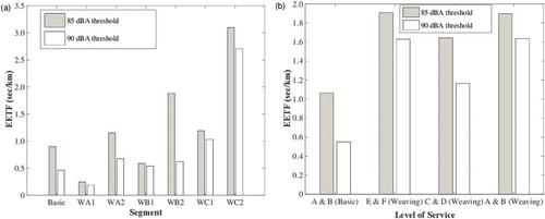
As shown in Figure 4a, the 8-hr 85 dB(A) EEFT on WC2 is the longest with about 3.2 sec/km, followed by 1.8 sec/km on WB2, then 1.25 sec/km on WA2 and WC1. The shortest EETF is observed on WA1 with 0.25 sec/km, which is almost 13 times shorter than the one on WC2. In comparison with the EETFs for 8-hr 85 dB(A), the EETFs for 8-hr 90 dB(A) are overall shorter on the seven segments. Likewise, the longest EETF is on WC2, followed by WC1 and WA2. The shortest EETF is found on WA1 with 0.2 sec/km, which is more than 4 times shorter than on the basic segment. In sum, the risk of the hazardous noise exposure is comparatively higher on WC2 and WB2, and tiny on WA1.

Figure 4b shows the hazardous exposure time factors under different level of traffic conditions on the seven segments. The EETF patterns for the thresholds 85 and 90 dB(A) are almost identical, and the EETFs on the basic segment are the lowest. It seems that the interior noise exposure is susceptible to the traffic conditions as well.

Besides, the EETFs during heavy traffic (LOD E and F) are similar to those during a free-flow mode at higher speeds (A and B), approximately 1.9 sec/km for 85 dB(A) exposure and 1.6 sec/km for 90 dB(A) exposure. During a mild traffic (C and D), the EETFs are the lowest in a weaving segment, with 1.6 and 1.2 sec/km for 85 and 90 dB(A) exposure levels, respectively, which are still 0.5 and 0.7 sec/km longer than driving on a basic segment under a free-flow mode. Thus, heavy ambient traffic and higher driving speeds could raise higher risk of hazardous interior noise exposure.

Hazard quotient

In principle, as long as the HQ is less than or equal to 1, no adverse effects resulted from the interior noise exposure on highways are expected. Figure 5 shows that the median levels of the HQs for the two thresholds are overall smaller than 1, about 0.4, and visible differences in the HQ levels between the thresholds are not observed. In other words, the hazard of adverse health effects resulted from the interior noise exposure is acceptable. Nevertheless, this exposure is still raising a load to the daily noise exposure for highway commuters. A noise monitoring study by Flamme et al. (2012) reported that median overall daily noise exposure levels or were 79 and 77 dB(A) among 286 participants in Kalamazoo County, Michigan, and 70% of them were exposed to an average noise level exceeding the noise limit 75 dB(A) recommended by EPA.

Figure 5. (a) Hazard quotient values for the threshold 85 dB(A) on segments. (b) Hazard quotient values for the threshold 90 dB(A) on segments.

Bagged decision tree–based in-vehicle noise emission models

Predictor importance

Eleven variables, including speed (v), acceleration rate (acc), vehicle-specific power (vsp), cLoad, aLoad, RPM, IRI, length of a weaving segment, type of a weaving segment/number of minimum lane change, accelerator pedal sensor D (AccD), and accelerator pedal sensor E (AccE), were obtainable from the driving tests, which could serve as predictors for the response of NED. The importance of the 11 predictor variables was evaluated by their OOB-permuted predictor delta error, the result of which is illustrated in Figure 6.

Figure 6. Importance of the 11 predictor variables for the bagged decision tree–based in-vehicle noise model.

The higher the score, the more important is the predictor for the NED estimate. Figure 6 shows that the 11 variables are important for the NED at different levels. IRI is the most important with the score of 6.5, whereas the scores for the other predictor variables range from 2 to 4. The least importance is the vsp with the score of 1.5, close to 2. All the 11 predictor variables are involved in the NED model as independent variables.

The number of grown trees for the noise model

For the NED model, the algorithm of bootstrap-aggregated (bagged) decision trees was applied. The number of grown trees is determined by the smallest OOB errors over 300 grown regression trees. A total of 30,898 valid data pairs were collected. Figure 7 displays an overview of the OOB regression errors from the training data set.

Figure 7. Out-of-bag regression error for 300 deep grown trees.

In Figure 7, the OOB error declines with the grown number of trees. When the tree number is greater than 125, the errors change rarely. Hence, 125 grown trees were determined to train a TreeBagger ensemble using the training data set. Table 3 shows the text description of the first 10 splits in the regression decision tree during the ensemble learning process.

Table 3. Text description of the first 10 splits in decision tree for regression.

Node	Text description
1.	if speed <62.7239 then node 2 elseif speed ≥62.7239 then node 3 else 33.9469%
2.	if speed <23.3969 then node 4 elseif speed ≥23.3969 then node 5 else 29.8813%
3.	if type <0.5 then node 6 elseif type ≥0.5 then node 7 else 37.0308%
4.	if speed <0.403899 then node 8 elseif speed ≥0.403899 then node 9 else 28.6712%
5.	if cLoad <10.5874% then node 10 elseif cLoad ≥10.5874% then node 11 else 31.9281%
6.	if speed <91.1465 then node 12 elseif speed ≥91.1465 then node 13 else 39.0558%
7.	if type <2.5 then node 14 elseif type ≥2.5 then node 15 else 35.7611%
8.	if IRI <3.66 then node 16 elseif IRI ≥3.66 then node 17 else 26.6343%
9.	if speed <16.3229 then node 18 elseif speed ≥16.3229 then node 19 else 28.9359%
10.	fit = 11.2171%
11.	if acc <0.906592 then node 20 elseif acc ≥0.906592 then node 21 else 31.9589%
12.	…

Note. *The type is defined by the number of minimum lane changes required for weaving.

In Table 3, there are 1 terminal node and 10 internal nodes at the first 10 splits. For the first split at the root node, if the speed is smaller than 62.7239 km/hr, the estimate comes to node 2. Otherwise, the estimate comes to node 3, or else the NED is 33.9469%. At node 2, the speed is further split into smaller than 23.3969 km/hr for node 4 and equal or greater than 23.3969 km/hr for node 5. At the node 5, the cLoad is split into smaller than 10.5874% for node 10 and equal or greater than 10.5874% for node 11. Node 10 is the terminal node. In other words, if the speed is between 23.3969 and 62.7239 km/hr and the cLoad is smaller than 10.5874%, the NED is 11.2171%. Similarly, other nodes are continuously split to reach their terminal nodes for NED estimation.

Accuracy of the NED model

The accuracy of the NED model is measured by the correlation coefficients and NRMSE between modeled and observed NED in the training data set as well as the validation data set. Figure 8 demonstrates a fitted regression line between the modeled NEDs and the observed NEDs in the training data set and validation data set.

Figure 8. Fitted regression lines for (a) training data set and (b) validation data set.

In Figure 8, the R value of the fitting regression line is 0.93 in the training as well as in the validation data sets, representing high correlation between the modeled NEDs and the observed NEDs. Further, the NRMSEs only increase 0.1% from 6.6% to 6.7% for the training and the validation data sets, respectively. This implies that the accuracy of the NED model is very stable and applicable to other data sets. Thus, the bagged decision tree–based NED model shows high predictive power.

Summary

An on-road driving test was conducted on 12 subjects on SH 288 in Houston, Texas, during peak and nonpeak hours of sunny weekdays, using one dedicated vehicle to collect vehicle maneuvering and engine operational information, pavement roughness, and real-time interior noise levels. Meanwhile, three types of weaving segment configuration on the test route were observed, in terms of the type and length of weaving segments. As a result, 11 predictors were retrieved from the collected data, including v, acc, vsp, cLoad, aLoad, RPM, IRI, AccD, AccE, and the length and type of a weaving segment indicated by the number of minimum lane change. The 11 predictors were synchronized and interpolated with their corresponding NED for feature selection process and aggregated for modeling data pairs. A bagged decision tree–based NED model was constructed with 30,898 valid data pairs. In addition, the hazardous exposure level of the vehicle interior noise on weaving segments was quantified to NED, L_ex, EETF, and HQ. The findings of this study are summarized as follows:

• Only a small portion of the measured vehicle interior noise exceeds the thresholds 85 and 90 dB(A) across the seven segments on the SH 288 freeway. The excessive noise is caused by heavy traffic passing or unexpected vibrations on rough pavement.

• Vehicle interior noise levels are sensitive to freeway traffic conditions and weaving configuration, in terms of the length and the type of weaving segment/number of minimum lane change.

• Heavy ambient traffic and higher driving speeds could raise higher risk of hazardous interior noise exposure.

• The interior noise exposure level is the lowest on Type A1 (one lane change, 370 m long) weaving segment and the highest on Type B1 (no lane change, 680 m long).

• Among the six weaving segments, the exposure likelihood of the interior noise is the highest on Type C2 (more than 2 lane changes, 920 m long) and the lowest on Type A1.

• Vehicle weaving on freeway accounts for 29–42% of the daily saturated noise exposure to 85 dB(A) for commuters.

• The risk of the freeway interior noise exposure is acceptable, indicating by an overall lower HQ (<1), about 0.4.

• The 11 predictors are important for the NED modeling at varied levels; the NED is the most sensitive to the pavement roughness, followed by engine loads and weaving segment designs, in terms of weaving length and the number of lane changes required.

• The constructed bagged decision tree–based NED model consists of 125 grown trees and shows high predictive power (R = 0.93, NRMSE < 6.7%).

Funding

The authors acknowledge the partial support for this research provided by the National Science Foundation (NSF) under grant 1137732 and the United States Tier 1 University Transportation Center TranLIVE no. DTRT12GUTC17/KLK900-SB-003. The opinions, findings, conclusions, and recommendations expressed in this material are those of the authors and do not necessarily reflect the views of the funding agencies.

Additional information

Funding

The authors acknowledge the partial support for this research provided by the National Science Foundation (NSF) under grant 1137732 and the United States Tier 1 University Transportation Center TranLIVE no. DTRT12GUTC17/KLK900-SB-003. The opinions, findings, conclusions, and recommendations expressed in this material are those of the authors and do not necessarily reflect the views of the funding agencies.

Notes on contributors

Qing Li

Qing Li is a research associate at the Innovative Transportation Research Institute at Texas Southern University, Houston, TX, USA.

Fengxiang Qiao

Fengxiang Qiao is a co-director and professor at the Innovative Transportation Research Institute at Texas Southern University, Houston, TX, USA.

Lei Yu

Lei Yu is a professor at Xuchang University, Xuchang City, Henan Province, People’s Republic of China, and a director and professor at the Innovative Transportation Research Institute at Texas Southern University, Houston, TX, USA.

Junqing Shi

Junqing Shi is an assistant professor at Zhejiang Normal University, Jinhua City, Zhejiang Province, People’s Republic of China, and a visiting scholar at the Innovative Transportation Research Institute, Texas Southern University, Houston, TX, USA.

References

- Breiman, L. 1996a. Out-of-bag estimation. http://citeseerx.ist.psu.edu/viewdoc/download? ( accessed April 16, 2017).
- Breiman, L. 1996b. Bagging predictors. Mach. Learn. 24:123–140. doi: 10.1007/BF00058655.
- Breiman, L., J. Friedman, R. Olshen, and C. Stone. 1984. Classification and Regression Trees. Boca Raton, FL: CRC Press.
- Brownlee, J. 2016. How to improve deep learning performance. http://machinelearningmastery.com/improve-deep-learning-performance/ ( accessed June 1, 2017).
- Chen, X. 2009. A comparison of decision tree and logistic regression model. https://www.mwsug.org/proceedings/2009/stats/MWSUG-2009-D02.pdf ( accessed June 1, 2017).
- Crocker, M.J. 2007. Handbook of Noise and Vibration Control. Hoboken, NJ: John Wiley & Sons.
- DriverSide. 2016. Glossary of Auto Terms. RPM. https://www.driverside.com/car-dictionary/rpm-9-204 (accessed July 29, 2016).
- Flamme, G.A., M. R. Stephenson, K. Deiters, A. Tatro, D. van Gessel, K. Geda, W. Krista, and K. McGregor. 2012. Typical noise exposure in daily life. Int, J. Audiol. 51(Suppl):S3–S11. doi: 10.3109/14992027.2011.635316.
- Forslöf, L., and H. Jones. 2015. Roadroid: Continuous road condition monitoring with smart phones. J. Civ. Eng. Archit. 9:485–496. doi: 10.17265/1934-7359/2015.04.012.
- Frigola-Alcade, R., 2015. Bayesian time series learning with gaussian processes. Ph.D. dissertation, University of Cambridge, Cambridge, UK.
- Hibbs, B.O., and R.M. Larson. 1996. Tire Pavement Noise and Safety Performance. Federal Highway Administration (FHWA), Final Report, FHW A-SA-96-068, May. https://www.fhwa.dot.gov/legsregs/directives/policy/sa_96_06.htm ( accessed November 2015).
- Kim, G.J., and N.J. Kim. 2000. The Identification of Tire-Induced Vehicle Interior Noise, SAE Technical Paper, 2000-05-0359. Seoul 2000 FISITA World Automotive Congress, June 12-15, 2000, Seoul, Korea
- Klein, R.D. 2003. How to win land development issues. Community and Environmental Defense Services. http://garivers.org/files/HTW.pdf ( accessed May 29, 2017).
- Li, Q., F. Qiao, and L. Yu. 2016a. Impacts of pavement types on in-vehicle noise and human health. J. Air Waste Manage. Assoc. 66:87–96. doi: 10.1080/10962247.2015.1119217.
- Li, Q., F. Qiao, Y. Qiao, and L. Yu 2016b. Impacts of traffic signal coordination on in-vehicle noises along an arterial road in Houston, USA. Paper presented at the 11th Asia Pacific Transportation Development Conference and the 29th ICTPA Annual Conference, Hsinchu, Taiwan, May 27–29. doi: 10.1061/9780784479810.022
- Li, Q., F. Qiao, and L. Yu. 2017. Risk assessment of in-vehicle noise pollution from highways. J. Environ. Pollut. Clim. Change 1:1000107.
- Liang, C.W., C.K. Ku, and J.J. Liang. 2012. Engine exhaust noise feedback to traffic flow and vehicle emission control on-road: A case study in Taichung City. Sustain. Environ. Res. 22:159–165.
- Liu, S., Q. Li, F. Qiao, J. Du, and L. Yu. 2017. Characterizing the relationship between carbon dioxide emissions and vehicle operating modes on roundabouts—A pilot test in a single lane entry roundabout. J. Environ. Pollut. Clim. Change 1:2:120.
- NoiseMeters Inc. 2017. TWA-time weighted average noise levels- and noise dose. https://www.noisemeters.com/help/osha/twa.asp ( accessed March 10, 2017).
- Occupational Safety and Health Administration. 1999. Regulations (Standards-29 CFR). Washington, DC: U.S. Government Printing Office.
- Park, J., L. Mongeau, and T. Siegmund. 2003. Effects of Window Seal Mechanical Properties on Vehicle Interior Noise. SAE Technical Paper 2003-01-1703. Warrendale, PA: SAE International. doi: 10.4271/2003-01-1703.
- Pearson, K. 1895. Notes on regression and inheritance in the case of two parents. Proc. R. Soc. Lond. 58:240–242. doi: 10.1098/rspl.1895.0041.
- Qiao, F., Q. Li, and L. Yu 2016. Neural network modeling of in-vehicle noise with different roadway roughness. Paper presented at the 29th ICTPA Annual Conference, Hsinchu, Taiwan, May 27–29, Paper no. 74. doi: 10.1061/9780784479810.020.
- SAE International. 1991. Surface Vehicle Standard. ISO 15031-5. Issued December 1991. http://standards.sae.org/j1979_201408/ (accessed July 29, 2016).
- Sandberg, U., and J.A. Ejsmont. 2002. Tyre/Road Noise Reference Book. Kisa, Sweden: Informex.
- Shorter, P. 2008. Recent advances in automotive interior noise prediction. SAE Technical Paper 2008-36-0592. Warrendale, PA: SAE International. doi: 10.4271/2008-36-0592
- Srivastava, T. 2015. Difference between machine learning & statistical modeling. https://www.analyticsvidhya.com/blog/2015/07/difference-machine-learning-statistical-modeling/ ( accessed June 1, 2017)
- Tingwall, E. 2015. They physics of engine notes, Or: Why a Toyota V-6 and Porsche Flat-Six sound so different. The science of engine sounds. http://www.caranddriver.com/features/this-is-why-various-engine-types-sound-so-different-feature ( accessed May 29, 2017).
- Transportation Research Board. 2000. Highway Capacity Manual, 4th ed. HCM 2000. Washington, DC: Transportation Research Board.
- U.S. Environmental Protection Agency. 1974. Information on Levels of Environmental Noise Requisite to Protect Public Health and Welfare with an Adequate Margin of Safety. EPA/ONAC 550/9-74-004. Washington, DC: U.S. Environmental Protection Agency.
- U.S. Environmental Protection Agency. 2011. NATA: Glossary of Terms. https://www.epa.gov/national-air-toxics-assessment/nata-glossary-terms ( accessed June 1, 2017).
- You, B., F. Qiao, and L. Yu. 2016. An exploration of CO2 emission models for horizontal curves on freeways. J. Environ. Sci. Eng. 6:2:1–8. doi: 10.4172/2165-784X.1000219.